library(readr)
library(dplyr)
library(ggplot2)
library(tidyverse)
library(leaflet)
library(tm)
library(tidytext)
library(wordcloud)

copenhagen <- read_csv('copenhagen_listings.csv')Airbnb Analysis in Copenhagen
Data Preparation & Exploration
The dataset contains information about Airbnb listings in Copenhagen, Denmark. Upon importing the data into R, we observed a significant number of missing values. To identify where these values occur, we used the colSums(is.na()) function, which enabled us to pinpoint missing data across columns and assess how best to handle them. By sorting these results in descending order, we prioritized columns with the most missing entries. We felt that values that are central to our exploratory and predictive analysis should have missing values removed, as imputing would potentially compromise these critical values. We chose to remove any rows that had NA values in price, review_scores_rating, and bedrooms. After this cleaning step, we retained 10,776 rows of information, plenty of data to run our analysis and a worthy compromise to ensure accuracy. For other columns with missing values, we applied targeted strategies. For example, we imputed missing values in the binary host_is_superhost column by assuming a value of FALSE for hosts without a recorded status. For the numeric variables bathrooms and beds, we replaced missing values with the median of each respective column. As for neighborhood_overview, we will simply exclude missing entries from any future analysis involving that variable. Remaining columns with missing values were deemed either nonessential for our analysis (e.g., license, host_neighbourhood, etc.), or had corresponding cleaned versions (e.g., neighbourhood and neighbourhood_cleansed). The has_availability field contained missing values. To impute these, we leveraged related variables: availability_30, availability_60, availability_90, and availability_365. If any of these showed more than 0 available days, we set has_availability to True. Furthermore, we found 2,630 records with no reviews, resulting in missing values for all review-related columns. We imputed review_scores_rating using the median value across the dataset. Overall, our cleaning approach allowed us to preserve a large portion of the dataset, while ensuring the data was complete for modeling purposes.
Missing Values
na_summary <- colSums(is.na(copenhagen)) %>%
  sort(decreasing = TRUE) %>%
  as.data.frame() %>%
  tibble::rownames_to_column(var = "Column") %>%
  rename(Missing_Count = ".") %>%
  mutate(Missing_Percent = round((Missing_Count / nrow(copenhagen)) * 100, 2))

print(na_summary)
copenhagen <- copenhagen %>%
filter(!is.na(price) & !is.na(review_scores_rating) & !is.na(bedrooms))
copenhagen <- copenhagen %>%
mutate(
host_is_superhost = ifelse(is.na(host_is_superhost), "FALSE", host_is_superhost)
)
copenhagen <- copenhagen %>%
group_by(room_type) %>%
mutate(
bathrooms = ifelse(is.na(bathrooms), median(bathrooms, na.rm = TRUE), bathrooms),
bedrooms = ifelse(is.na(bedrooms), median(bedrooms, na.rm = TRUE), bedrooms),
beds = ifelse(is.na(beds), median(beds, na.rm = TRUE), beds),
price = ifelse(is.na(price), median(price, na.rm = TRUE), price)
) %>%
ungroup()
# if property available in N days => has_availability is True
copenhagen$has_availability[is.na(copenhagen$has_availability)] <- ifelse(
is.na(copenhagen$has_availability) &
rowSums(copenhagen[is.na(copenhagen$has_availability), c("availability_30", "availability_60", "availability_90", "availability_365")] > 0, na.rm = TRUE) > 0, TRUE, FALSE)
# 2630 records with no_review
copenhagen$reviews_per_month[copenhagen$number_of_reviews == 0] <- 0
# set Median value for NAs in review related columns
copenhagen$review_scores_rating <- replace_na(copenhagen$review_scores_rating,
median(copenhagen$review_scores_rating, na.rm = TRUE))
copenhagen$review_scores_location <- replace_na(copenhagen$review_scores_location,
median(copenhagen$review_scores_location, na.rm = TRUE))
copenhagen$review_scores_value <- replace_na(copenhagen$review_scores_value,
median(copenhagen$review_scores_value, na.rm = TRUE))Summary Statistics
table(copenhagen$neighbourhood_cleansed)
                Amager st               Amager Vest                Bispebjerg
                      839                       989                       478
             Brnshj-Husum             Frederiksberg                  Indre By
                      167                      1130                      1818
                  Nrrebro                   sterbro                     Valby
                     1764                      1109                       381
                   Vanlse Vesterbro-Kongens Enghave
                      242                      1859
We first used table to see the different neighborhoods and how many listings were in each one. There are 11 neighborhoods and we chose to keep them all as these are the 10 municipal districts of Copenhagen plus Frederiksberg, which is its center. It felt like these would all be distinct and not too overwhelming to look at. We also knew we were going to want to look at price so made sure to convert it to a numeric and remove the dollar signs and commas.
copenhagen$price <- as.numeric(gsub("[$,]", "", copenhagen$price))
avgpricebyneighborhood <- copenhagen %>% group_by(neighbourhood_cleansed) %>%
  summarise(mean(price))
avgpricebyneighborhood
# A tibble: 11 × 2
neighbourhood_cleansed `mean(price)`
<chr> <dbl>
1 Amager Vest 1332.
2 Amager st 1220.
3 Bispebjerg 937.
4 Brnshj-Husum 959.
5 Frederiksberg 1329.
6 Indre By 1887.
7 Nrrebro 1206.
8 Valby 1021.
9 Vanlse 1041.
10 Vesterbro-Kongens Enghave 1365.
11 sterbro 1421.The first statistic we chose to look at was the average price per night for a listing in each neighborhood. We see here that the average price for listings in Indre By are basically double those in Bispebjerg and Brnshj-Husum. There’s quite a big range across the neighborhoods, so our takeaway is that different neighborhoods are more expensive—we don’t know why yet though, it could be due to demand or popularity or any other factor.
avgaccomodatesbyneighborhood <- copenhagen %>% group_by(neighbourhood_cleansed) %>%
  summarise(mean(accommodates))
avgaccomodatesbyneighborhood
# A tibble: 11 × 2
neighbourhood_cleansed `mean(accommodates)`
<chr> <dbl>
1 Amager Vest 3.58
2 Amager st 3.48
3 Bispebjerg 3.05
4 Brnshj-Husum 3.96
5 Frederiksberg 3.32
6 Indre By 3.76
7 Nrrebro 3.01
8 Valby 3.43
9 Vanlse 3.83
10 Vesterbro-Kongens Enghave 3.20
11 sterbro 3.29The next stat we chose to look at was the average number of people accommodated in each listing, or basically how many people can fit, by neighborhood. There is much less variety here with Nrrebro having a mean of approximately 3 and Brnshj-Husum having a mean of almost 4. Part of the reason for the smaller range is likely due to the fact that these are all still in the same city—it’s not likely for some neighborhoods to have properties accommodating 20 while some only accommodate 1.
propertytypebyneighborhood <- copenhagen %>% count(neighbourhood_cleansed, property_type,
                                                   sort = TRUE)
propertytypebyneighborhood
# A tibble: 197 × 3
neighbourhood_cleansed property_type n
<chr> <chr> <int>
1 Indre By Entire rental unit 1108
2 Nrrebro Entire rental unit 1107
3 Vesterbro-Kongens Enghave Entire rental unit 1056
4 sterbro Entire rental unit 691
5 Frederiksberg Entire rental unit 655
6 Vesterbro-Kongens Enghave Entire condo 573
7 Nrrebro Entire condo 517
8 Amager Vest Entire rental unit 457
9 Amager st Entire rental unit 429
10 Indre By Entire condo 411
# ℹ 187 more rowsNext, we looked at grouping by both property type and neighborhood. As we saw earlier by using table, Indre By has around 1800 listings. 1108 of them are entire rental units, this is the most common combination of neighborhood and property type. Entire rental units seem to make up a bulk of the listings in Copenhagen overall, accounting for the entire top 5 common combinations. By the time we even get to the 20th common combination, these are much rarer property types with less than 100 in each neighborhood.
superhostbyneighborhood <- copenhagen %>% group_by(neighbourhood_cleansed) %>%
  summarise(total=n(), superhost = sum(host_is_superhost == TRUE),
            percent = (superhost/total) * 100)
print(superhostbyneighborhood)
# A tibble: 11 × 4
neighbourhood_cleansed total superhost percent
<chr> <int> <int> <dbl>
1 Amager Vest 989 180 18.2
2 Amager st 839 153 18.2
3 Bispebjerg 478 77 16.1
4 Brnshj-Husum 167 32 19.2
5 Frederiksberg 1130 184 16.3
6 Indre By 1818 422 23.2
7 Nrrebro 1764 257 14.6
8 Valby 381 72 18.9
9 Vanlse 242 46 19.0
10 Vesterbro-Kongens Enghave 1859 360 19.4
11 sterbro 1109 164 14.8Next, we looked at the percentage of listings by superhosts per neighborhood. Indre By has the highest number of listings but it also has the highest superhost percentages with 23.21%. By contrast, Nrrerbro only has 14.57% even though it has a similar number of listings. Airbnb superhost status is something determined by Airbnb and is a status given to hosts that are top-rated and experienced. This suggests that either Indre By listings are reliable due to their superhosts, or it could also mean it’s a popular area letting the hosts get more experience. Knowing this is the most expensive average neighborhood, our takeaway is that it’s a bit of both. The price is likely due to popularity, and the hosts likely thus have competition so are more focused on making sure the guests have good experiences.
ratingbyneighborhood <- copenhagen %>% group_by(neighbourhood_cleansed) %>%
  summarise(mean(review_scores_rating))
ratingbyneighborhood
# A tibble: 11 × 2
neighbourhood_cleansed `mean(review_scores_rating)`
<chr> <dbl>
1 Amager Vest 4.84
2 Amager st 4.81
3 Bispebjerg 4.80
4 Brnshj-Husum 4.80
5 Frederiksberg 4.85
6 Indre By 4.80
7 Nrrebro 4.83
8 Valby 4.82
9 Vanlse 4.79
10 Vesterbro-Kongens Enghave 4.85
11 sterbro 4.84Finally, we looked at the average review_scores_rating which we interpreted as the overall rating score. Here, there is again not a huge range with the lowest score being 4.79 and the highest being 4.85. Our takeaway here is that most people are having positive experiences, but we do need to consider that perhaps the only people who are reviewing are those happy while those unhappy may be filing complaints with Airbnb instead. Alternatively, some people may feel bad leaving anything lower than a 4 knowing these aren’t really corporations.
Data Visualization
To begin our visualization process, we earlier cleaned the Copenhagen dataset by removing punctuation from the price column and converting it to numeric data. Additionally, we filtered the data to exclude any listings priced over 25,000 DKK per night, as these extreme outliers would skew our visualizations and detract from more meaningful trends.
#clean price column
copenhagen <- copenhagen %>% filter(price < 25000)

#boxplot of price in top 10
ggplot(copenhagen, aes(x = fct_reorder(neighbourhood_cleansed, price, .fun = median),
                       y = price)) +
  geom_boxplot(fill = "cornflowerblue") +
  coord_flip() +
  labs(title = "Price Distribution by Neighborhood",
       x = "Neighborhood", y = "Price (DKK)")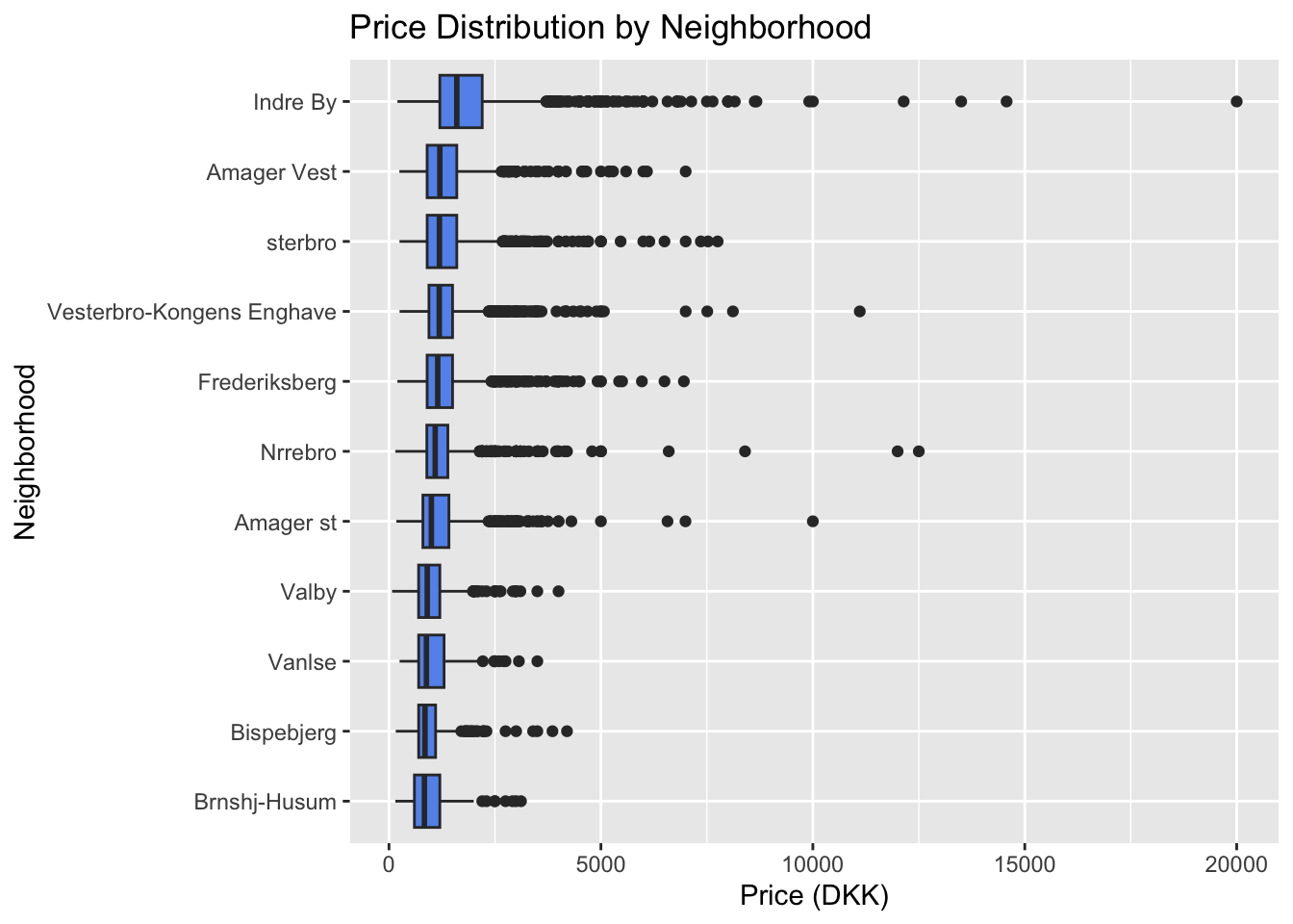
Our first visualization is a boxplot comparing listing price distributions across the eleven Copenhagen neighborhoods. Indre By (which translates to “Inner City”) exhibits both the highest median price and the widest price range, likely due to its central, high-demand location. Other neighborhoods with notable outliers above 10,000 DKK include Vesterbro/Kongens Enghave, Nørrebro (presented as “Nrrebro” in the data due to special character limitations), and Amager Øst (“Amager st” in the data). Each of these neighborhoods borders the water, suggesting that waterfront properties may be commanding a premium, due to location and aesthetic. In contrast, Bispebjerg and Brønshøj-Husum (“Brnshj-Husum”) show lower median prices and fewer extreme outliers, indicating more affordable options. These neighborhoods are farther from the harbor and city center, making them less desirable for tourists.
#group by neighborhood and superhost
superhost_breakdown <- copenhagen %>%
  group_by(neighbourhood_cleansed, host_is_superhost) %>%
  summarise(count = n(), .groups = "drop") %>%
  group_by(neighbourhood_cleansed) %>%
  mutate(percent = count / sum(count) * 100)


#plot by number of listings and breakdown of super or not
ggplot(superhost_breakdown, aes(x = reorder(neighbourhood_cleansed, -count), y = count, fill = host_is_superhost)) +
  geom_col() +
  geom_text(
    aes(label = paste0(round(percent), "%")),
    position = position_stack(vjust = 0.5),
    color = "white",
    size = 2) +
  coord_flip() +
  labs(
    title = "Superhost Composition by Neighborhood",
    x = "Neighborhood",
    y = "Number of Listings",
    fill = "Superhost") +
  scale_fill_manual(values = c("FALSE" = "cornflowerblue", "TRUE" = "salmon"))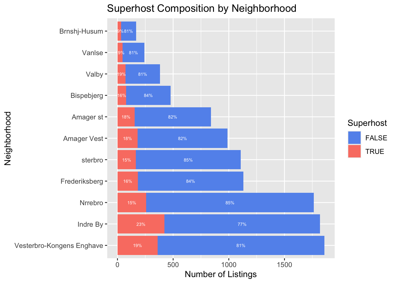
Our second visualization is a stacked bar plot showing the percentage of Superhosts by neighborhood, with the total number of listings displayed along the x-axis. Superhost percentages generally fall within the 15–20% range, with Indre By again standing out at 23%. Indre By also has the second-highest number of listings, reinforcing its competitiveness and potentially explaining the higher concentration of Superhosts, the high number of listings also explains the wide range of pricing seen in the boxplot. Vesterbro/Kongens Enghave, Indre By, and Nørrebro also have significantly more listings than other neighborhoods, reflecting their popularity among tourists. On the other hand, Brønshøj-Husum and Vanløse have the lowest Superhost rates at 9%, aligning with their lower pricing and likely simpler accommodation offerings.
# distribution of reviews with proportions and mean
ggplot(copenhagen, aes(x = review_scores_rating)) +
  geom_histogram(
    binwidth = 0.2,
    fill = "cornflowerblue",
    color = "salmon") +
  stat_bin(
    binwidth = 0.2,
    geom = "text",
    aes(label = scales::percent(after_stat(count / sum(count)), accuracy = .1)),
    vjust = -0.5,
    color = "black",
    size = 2) +
  geom_vline(
    xintercept = mean(copenhagen$review_scores_rating, na.rm = TRUE),
    color = "orchid",
    linetype = "dashed",
    size = 1) +
  labs(
    title = "Distribution of Review Scores",
    x = "Review Score",
    y = "Number of Listings") +
  theme_minimal()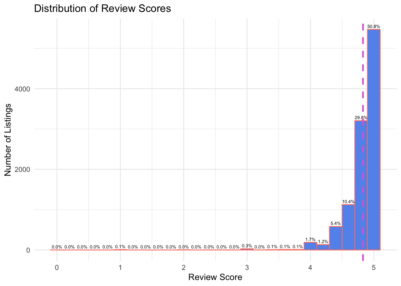
The third visualization is a histogram showing the distribution of review scores across all listings. Review scores are heavily left-skewed, with almost all reviews clustered between 4.5 and 5.0. The mean review score, marked by a dashed orchid line on the plot, is 4.82. Each bar is labeled with the percentage of total listings it represents, helping highlight how concentrated the reviews are in the highest ranges. There is a small uptick (only around .3%) in reviews around 3.0 likely represents guests who had neutral experiences, possibly correlating with lower-cost, lower-amenity listings. While this diagram suggests almost exclusive positive reviews, this is possibly due to the subjective nature of voluntary reviewing. Guests who felt incredibly satisfied with their stays are more likely to share their happy feelings than those who simply felt neutral, or unhappy. It would be interesting to explore if Airbnb filters out negative reviews, as the near total absence of low scores seems somewhat unlikely.
mean(copenhagen$review_scores_rating)[1] 4.828895#price vs review scatterplot
ggplot(copenhagen, aes(x = review_scores_rating, y = price)) +
geom_point(alpha = 0.3, color = "orchid") +
geom_smooth(method = "lm", se = FALSE, color = "black", linetype = "dashed") +
labs(
title = "Price vs. Review Score",
x = "Review Score",
y = "Price (DKK)")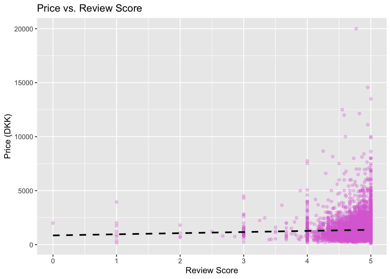
The fourth visualization is a scatterplot examining the relationship between price and review score, with a dashed line representing the line of best fit. While the trend line does have a slight positive incline, it is nearly flat suggesting that a higher price does not correlate to a higher review score. This indicates that other factors (such as location or amenities) likely correlate more to guest satisfaction than value. It is interesting to note that all the listings with a per night price of 10,000 DKK or more received a review score of 4.5 or greater. This indicates an incredibly premium price does tend to correlate with a satisfied guest.
#density plot of price by room type
ggplot(copenhagen, aes(x = price, fill = room_type)) +
  geom_density(alpha = 0.4) +
  labs(
    title = "Price Distribution by Room Type",
    x = "Price (DKK)",
    y = "Density",
    fill = "Room Type") +
  xlim(0, 3000) +
  theme_minimal() +
  scale_fill_brewer(palette = "Set2")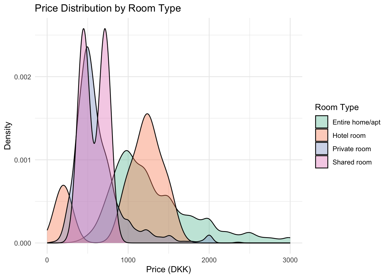
Finally, the fifth visualization is a density plot illustrating price distributions across different room types. As expected, entire homes/apartments have the highest price range, reflecting one of Airbnb’s main benefits compared to hotels. Hotel rooms show a spike in the mid-to-high range, with little variation at the higher end but a small second spike at the very low end. Perhaps these are hostel style accommodations that are being referred to as hotel rooms, as hotels are typically Airbnb’s main competitors. Private rooms and shared rooms are concentrated at lower price points, likely catering to students and budget-conscious travelers such as backpackers. Overall, room type and location are likely the strongest predictors of listing price.
Mapping
leaflet(data = copenhagen) %>%
  addTiles() %>%
  addCircleMarkers(
    ~longitude, ~latitude,
    radius = .1,
    color = "#6A5ACD",
    fillOpacity = 0.2) %>%
  setView(lng = mean(copenhagen$longitude),
          lat = mean(copenhagen$latitude),
          zoom = 12)
The interactive map built with the Leaflet package shows the geographic distribution of Airbnb listings across Copenhagen. The map confirms what the neighborhood listings bar plot displayed in Part III, listings are highly concentrated in Vesterbro/Kongens Enghave, Indre By, and Nørrebro, as these areas are located in close proximity to both the city center and the harbor. As one moves farther from the city center, the density of listings decreases noticeably, with much sparser coverage in outlying areas that are likely residential suburbs. Additionally, there are very few listings directly along the harborfront, likely due to commercial zones for cargo and cruise ships. The map suggests that Airbnb hosts strategically locate their listings near Copenhagen’s main attractions, shopping areas, restaurants, historical sites, and public transportation. The density also drops off significantly in suburban residential areas, which are less accessible to tourists and are likely populated primarily by full-time local residents. Finally, several large patches of open land visible on the map correspond to Copenhagen’s protected parks and green spaces. The lack of Airbnb listings in these areas reflects a cultural phenomenon in the region. Copenhagen, and Denmark as a whole, are well known for their emphasis on sustainability and their strong commitment to preserving the environment. This is reflected in strict land use regulations that prevent commercial developments, including Airbnb listings, from encroaching on protected natural spaces.
Wordcloud
Unigram wordcloud
copenhagen_text <- copenhagen %>%
  filter(!is.na(neighborhood_overview)) %>%
  pull(neighborhood_overview) %>%
  iconv(from = "UTF-8", to = "ASCII", sub = "") %>%
  paste(collapse = " ")

copenhagen_text_df <- data.frame(text = copenhagen_text)

copenhagen_text_clean <- copenhagen_text_df %>%
  unnest_tokens(word, text) %>%
  filter(!word %in% stopwords("english")) %>%
  filter(!word %in% c("copenhagen", "area", "neighborhood", "location", "br"))

copenhagen_freq <- copenhagen_text_clean %>%
  count(word, sort = TRUE)

wordcloud(
  words = copenhagen_freq$word,
  freq = copenhagen_freq$n,
  max.words = 100,
  colors = brewer.pal(8, "Dark2"),
  random.order = TRUE)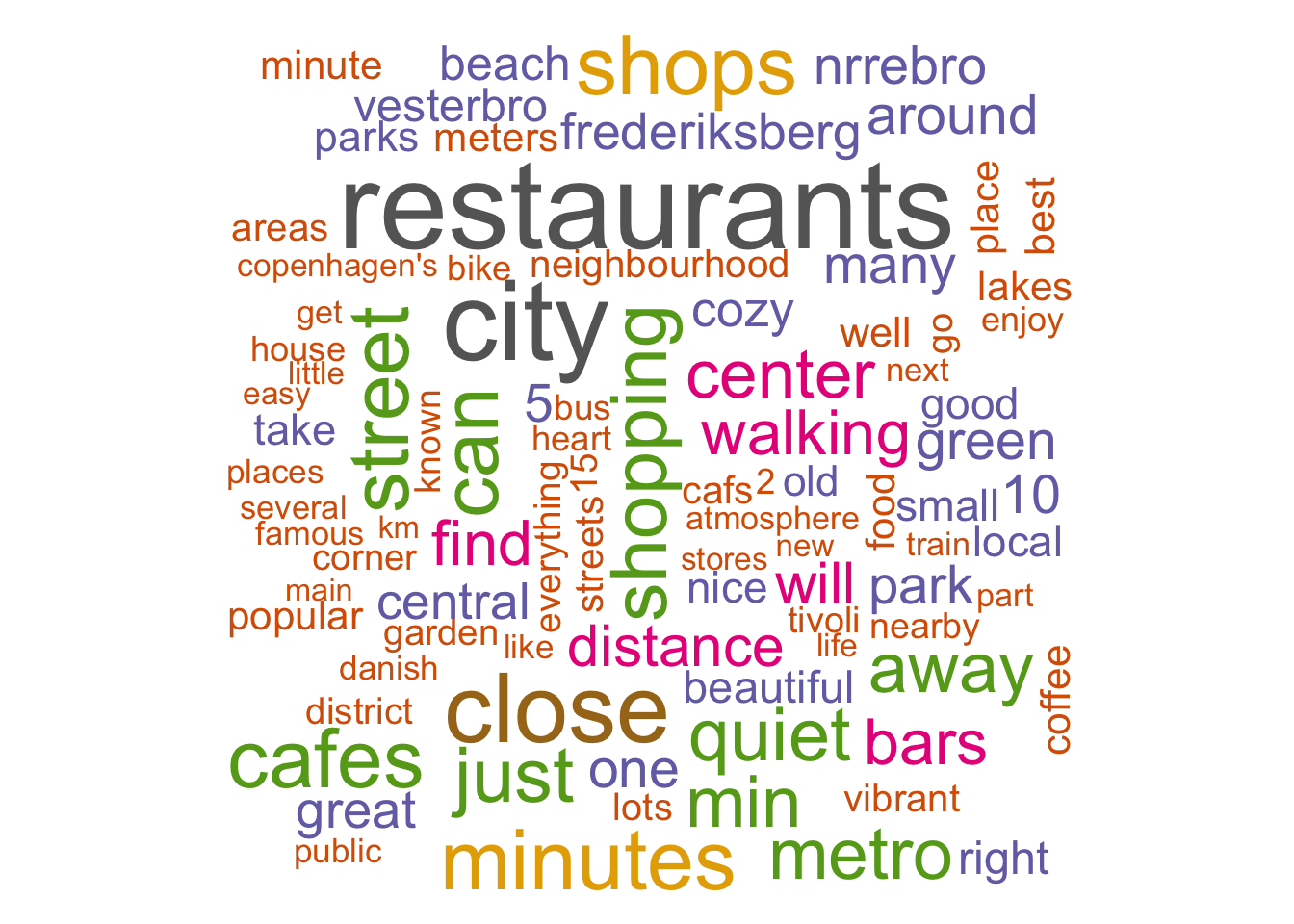
The wordcloud visualization is generated from the neighborhood overview descriptions from the Airbnb listings. The most common term is restaurants, followed by words like walk, located, close, minutes, shopping, and metro. These terms emphasize proximity and convenience, giving guests the impression of walkability and easy access to amenities. This again confirms the popularity of listings near Copenhagen’s city center, as guests tend to prioritize connection to attractions and transportation. Copenhagen is renowned for its public transportation system and overall walkability, making it strategic for hosts to highlight these traits in their descriptions.
Descriptive words such as quiet, cozy, charming, and vibrant also appear prominently, reflecting the hosts’ efforts to market a welcoming and pleasant atmosphere. The Danish concept of hygge is centered around creating warm, cozy environments and enjoying simple pleasures, particularly in the winter months. Given that Copenhagen experiences very short daylight hours in winter (an average of just one hour of sunshine in December), emphasizing a cozy and comfortable environment is an effective way for hosts to appeal to guests seeking an authentic hygge experience. The hosts’ use of these descriptive words evokes a strong sense of hygge, making their listings even more attractive to travelers looking for comfort and community during the darker months.
Bigram cloud
bigrams <- copenhagen_text_df %>%
  unnest_tokens(bigram, text, token = "ngrams", n = 2)

bigrams_separated <- bigrams %>%
  separate(bigram, into = c("word1", "word2"), sep = " ")

bigrams_filtered <- bigrams_separated %>%
  filter(!word1 %in% stopwords("english"),
         !word2 %in% stopwords("english"),
         !word1 %in% c("copenhagen", "br"),
         !word2 %in% c("copenhagen", "br"))

bigrams_united <- bigrams_filtered %>%
  unite(bigram, word1, word2, sep = " ")
bigram_freq <- bigrams_united %>%
  count(bigram, sort = TRUE)

wordcloud(
  words = bigram_freq$bigram,
  freq = bigram_freq$n,
  max.words = 100,
  colors = brewer.pal(8, "Dark2"),
  random.order = FALSE)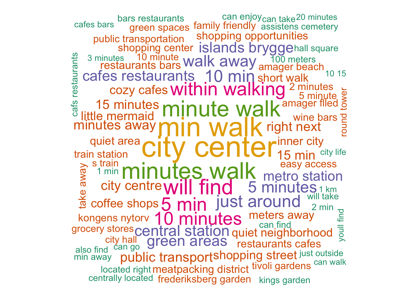
To add further context, we also generated a second wordcloud based on bigrams from the neighborhood overview descriptions. While not explicitly required for the assignment, we felt the bigram visualization provided additional insight into features that hosts highlight in their listings. Common phrases such as city center, minute walk, metro station, and central station once again emphasize the value of proximity and accessibility. This reinforces the recurring theme that guests place a very high value on location and walkability. The more a host can market the convenience and centrality of their listing, the more it will likely appeal to potential guests. Additionally, the bigram cloud included Copenhagen-specific tourism features such as Islands Brygge, meatpacking district, and the Little Mermaid, suggesting that hosts emphasize proximity to famous landmarks when marketing their properties.
Prediction
library(reshape2)set.seed(699)
train.indexpred <- sample(c(1:nrow(copenhagen)), nrow(copenhagen)*0.6)
train.df <- copenhagen[train.indexpred,]
valid.df <- copenhagen[-train.indexpred,]
train.df = train.df %>% select(19,29,33:36,38,39,41,52:55,57:59,62:68,70)
train.df$host_is_superhost <- as.factor(train.df$host_is_superhost)
train.df$neighbourhood_cleansed <- as.factor(train.df$neighbourhood_cleansed)
train.df$property_type <- as.factor(train.df$property_type)
train.df$room_type <- as.factor(train.df$room_type)
train.df$instant_bookable <- as.factor(train.df$instant_bookable)To build our multiple linear regression model, we first began with dividing our data into a training and validation set. Then, we looked at the dataset and dataset description and selected the variables that we thought would be relevant, excluding things like url, host profile photo, etc… landing on the following variables:
colnames(train.df) [1] "host_is_superhost" "neighbourhood_cleansed"
[3] "property_type" "room_type"
[5] "accommodates" "bathrooms"
[7] "bedrooms" "beds"
[9] "price" "availability_30"
[11] "availability_60" "availability_90"
[13] "availability_365" "number_of_reviews"
[15] "number_of_reviews_ltm" "number_of_reviews_l30d"
[17] "review_scores_rating" "review_scores_accuracy"
[19] "review_scores_cleanliness" "review_scores_checkin"
[21] "review_scores_communication" "review_scores_location"
[23] "review_scores_value" "instant_bookable" # Compute correlation matrix
cordata = train.df %>% select(5:8,10:23)
cormat <- cor(cordata, use = "pairwise.complete.obs")
# Convert to long format
melted_cormat <- melt(cormat)
# Heatmap
ggplot(melted_cormat, aes(Var1, Var2, fill = value)) +
geom_tile(color = "white") +
scale_fill_gradient2(low = "blue", high = "red", mid = "white",
midpoint = 0, limit = c(-1,1), space = "Lab",
name = "Correlation") +
theme_minimal() +
theme(axis.text.x = element_text(angle = 45, vjust = 1, hjust=1)) +
coord_fixed() +
labs(title = "Correlation Heatmap")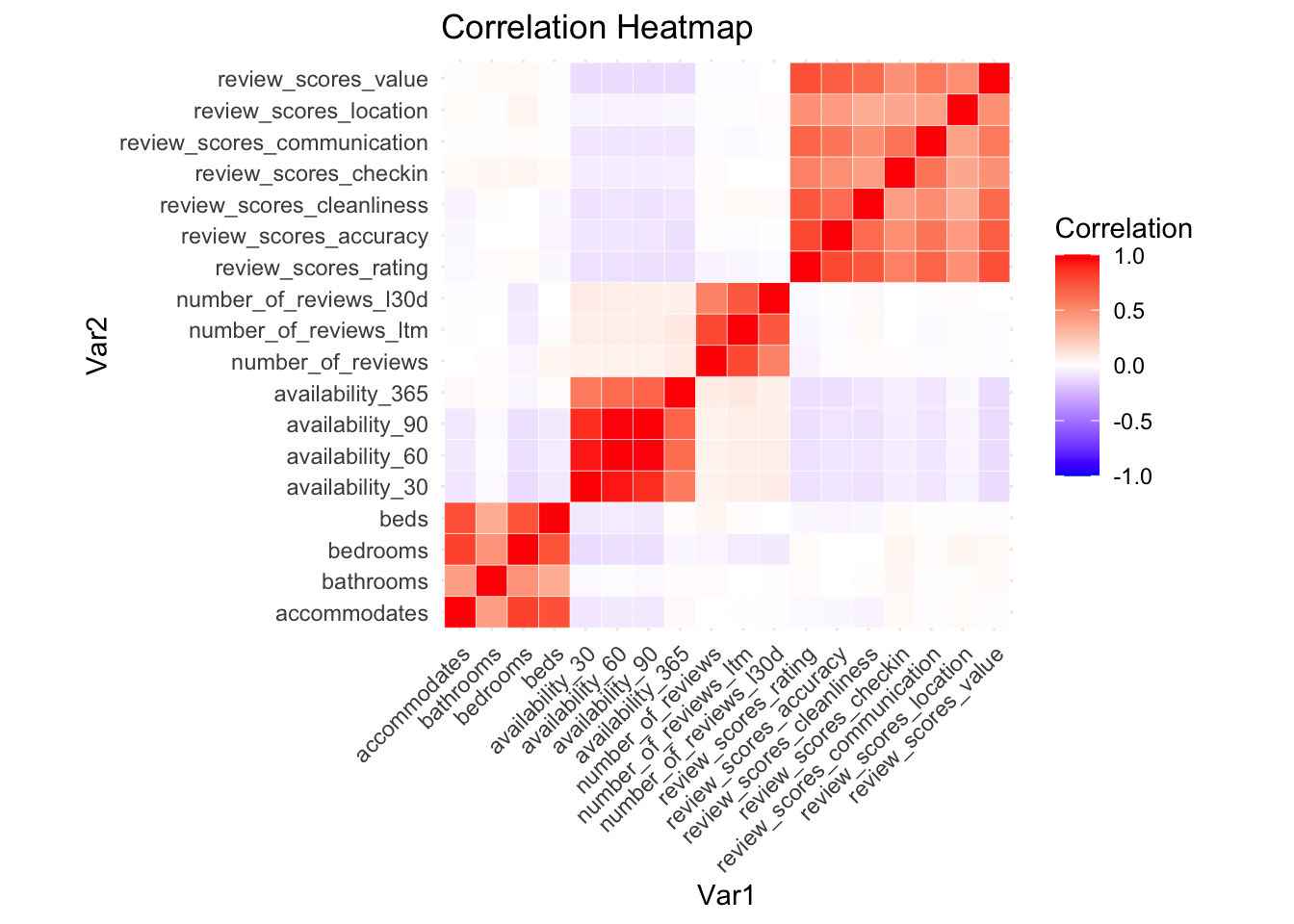
We then looked at correlation to try and avoid collinearity. We removed bedrooms, beds, availability_60, availability_90, number_of_reviews, and review_scores_value due to strong correlations with other variables.
train.df = subset(train.df, select=-c(
  bedrooms, beds, availability_60, availability_90, number_of_reviews_ltm,review_scores_value))
Finally, we used backwards elimination to remove some more variables.
mlrmodel <-lm(price ~ .,
              data = train.df)

mlrmodel.step <- step(mlrmodel, direction = "backward")
Start: AIC=84676.9
price ~ host_is_superhost + neighbourhood_cleansed + property_type +
room_type + accommodates + bathrooms + availability_30 +
availability_365 + number_of_reviews + number_of_reviews_l30d +
review_scores_rating + review_scores_accuracy + review_scores_cleanliness +
review_scores_checkin + review_scores_communication + review_scores_location +
instant_bookable
Df Sum of Sq RSS AIC
- room_type 1 130507 3107648307 84675
- review_scores_rating 1 453113 3107970912 84676
- review_scores_checkin 1 625371 3108143171 84676
- number_of_reviews 1 895824 3108413624 84677
<none> 3107517800 84677
- review_scores_location 1 1029241 3108547040 84677
- host_is_superhost 1 2782925 3110300724 84681
- review_scores_communication 1 2964072 3110481872 84681
- instant_bookable 1 2993626 3110511426 84681
- review_scores_accuracy 1 3539682 3111057481 84682
- property_type 38 41170228 3148688028 84686
- review_scores_cleanliness 1 8214675 3115732475 84692
- availability_365 1 19980311 3127498110 84716
- number_of_reviews_l30d 1 29940576 3137458376 84737
- availability_30 1 39110394 3146628193 84756
- bathrooms 1 116410784 3223928583 84913
- neighbourhood_cleansed 10 272114038 3379631838 85199
- accommodates 1 534452716 3641970515 85700
Step: AIC=84675.18
price ~ host_is_superhost + neighbourhood_cleansed + property_type +
accommodates + bathrooms + availability_30 + availability_365 +
number_of_reviews + number_of_reviews_l30d + review_scores_rating +
review_scores_accuracy + review_scores_cleanliness + review_scores_checkin +
review_scores_communication + review_scores_location + instant_bookable
Df Sum of Sq RSS AIC
- review_scores_rating 1 453500 3108101807 84674
- review_scores_checkin 1 618935 3108267242 84674
- number_of_reviews 1 893680 3108541987 84675
<none> 3107648307 84675
- review_scores_location 1 1044197 3108692504 84675
- host_is_superhost 1 2778062 3110426369 84679
- review_scores_communication 1 2956766 3110605073 84679
- instant_bookable 1 3057900 3110706207 84680
- review_scores_accuracy 1 3552931 3111201238 84681
- review_scores_cleanliness 1 8221882 3115870189 84690
- availability_365 1 19968925 3127617232 84715
- number_of_reviews_l30d 1 30017066 3137665373 84735
- availability_30 1 39142076 3146790383 84754
- property_type 40 120583502 3228231809 84841
- bathrooms 1 116384097 3224032404 84911
- neighbourhood_cleansed 10 272005324 3379653631 85197
- accommodates 1 534555892 3642204199 85699
Step: AIC=84674.12
price ~ host_is_superhost + neighbourhood_cleansed + property_type +
accommodates + bathrooms + availability_30 + availability_365 +
number_of_reviews + number_of_reviews_l30d + review_scores_accuracy +
review_scores_cleanliness + review_scores_checkin + review_scores_communication +
review_scores_location + instant_bookable
Df Sum of Sq RSS AIC
- review_scores_checkin 1 517584 3108619391 84673
- number_of_reviews 1 826583 3108928390 84674
- review_scores_location 1 862402 3108964209 84674
<none> 3108101807 84674
- host_is_superhost 1 2689241 3110791048 84678
- review_scores_accuracy 1 3147032 3111248839 84679
- instant_bookable 1 3237881 3111339688 84679
- review_scores_communication 1 3891683 3111993490 84680
- review_scores_cleanliness 1 8140360 3116242168 84689
- availability_365 1 20002118 3128103925 84714
- number_of_reviews_l30d 1 30155144 3138256951 84735
- availability_30 1 39234663 3147336470 84753
- property_type 40 120308115 3228409923 84840
- bathrooms 1 116336832 3224438639 84910
- neighbourhood_cleansed 10 273403509 3381505316 85199
- accommodates 1 534913347 3643015154 85698
Step: AIC=84673.2
price ~ host_is_superhost + neighbourhood_cleansed + property_type +
accommodates + bathrooms + availability_30 + availability_365 +
number_of_reviews + number_of_reviews_l30d + review_scores_accuracy +
review_scores_cleanliness + review_scores_communication +
review_scores_location + instant_bookable
Df Sum of Sq RSS AIC
- number_of_reviews 1 790343 3109409734 84673
<none> 3108619391 84673
- review_scores_location 1 1094951 3109714342 84673
- host_is_superhost 1 2721272 3111340662 84677
- instant_bookable 1 3197921 3111817312 84678
- review_scores_communication 1 3382674 3112002065 84678
- review_scores_accuracy 1 3413615 3112033006 84678
- review_scores_cleanliness 1 8518034 3117137425 84689
- availability_365 1 20020743 3128640134 84713
- number_of_reviews_l30d 1 30210300 3138829691 84734
- availability_30 1 39201473 3147820864 84752
- property_type 40 120098923 3228718314 84838
- bathrooms 1 116399996 3225019387 84909
- neighbourhood_cleansed 10 272904291 3381523682 85197
- accommodates 1 535777278 3644396669 85699
Step: AIC=84672.84
price ~ host_is_superhost + neighbourhood_cleansed + property_type +
accommodates + bathrooms + availability_30 + availability_365 +
number_of_reviews_l30d + review_scores_accuracy + review_scores_cleanliness +
review_scores_communication + review_scores_location + instant_bookable
Df Sum of Sq RSS AIC
<none> 3109409734 84673
- review_scores_location 1 1160816 3110570550 84673
- host_is_superhost 1 2230932 3111640666 84675
- instant_bookable 1 3122952 3112532686 84677
- review_scores_communication 1 3394669 3112804403 84678
- review_scores_accuracy 1 3403513 3112813247 84678
- review_scores_cleanliness 1 8531773 3117941507 84689
- availability_365 1 19743820 3129153554 84712
- availability_30 1 39616788 3149026522 84753
- number_of_reviews_l30d 1 44775227 3154184960 84763
- property_type 40 123083939 3232493672 84844
- bathrooms 1 116222176 3225631909 84908
- neighbourhood_cleansed 10 272201524 3381611258 85195
- accommodates 1 535031737 3644441471 85697The regression equation that the model generated is extremely long because of the categorical variables that remain. It is the intercept (134.7556) + the product of each intercept times the value for each variable (ex:212.7862 * the number of people the listing can accommodate).
summary(mlrmodel.step)
Call:
lm(formula = price ~ host_is_superhost + neighbourhood_cleansed +
    property_type + accommodates + bathrooms + availability_30 +
    availability_365 + number_of_reviews_l30d + review_scores_accuracy +
    review_scores_cleanliness + review_scores_communication +
    review_scores_location + instant_bookable, data = train.df)

Residuals:
    Min      1Q  Median      3Q     Max
-1954.1  -312.0   -78.4   171.3 16721.0

Coefficients:
                                                  Estimate Std. Error t value
(Intercept)                                     -2.688e+02  4.749e+02  -0.566
host_is_superhostTRUE                            5.082e+01  2.372e+01   2.143
neighbourhood_cleansedAmager Vest                6.346e+01  4.271e+01   1.486
neighbourhood_cleansedBispebjerg                -1.495e+02  5.180e+01  -2.885
neighbourhood_cleansedBrnshj-Husum              -3.287e+02  7.688e+01  -4.275
neighbourhood_cleansedFrederiksberg              1.301e+02  4.146e+01   3.138
neighbourhood_cleansedIndre By                   5.860e+02  3.895e+01  15.045
neighbourhood_cleansedNrrebro                    7.991e+01  3.866e+01   2.067
neighbourhood_cleansedsterbro                    1.275e+02  4.160e+01   3.065
neighbourhood_cleansedValby                     -1.999e+02  5.557e+01  -3.597
neighbourhood_cleansedVanlse                    -2.944e+02  6.791e+01  -4.335
neighbourhood_cleansedVesterbro-Kongens Enghave  1.355e+02  3.827e+01   3.541
property_typeEntire bungalow                    -1.421e+03  5.708e+02  -2.489
property_typeEntire cabin                       -8.787e+02  5.718e+02  -1.537
property_typeEntire condo                       -7.803e+02  4.045e+02  -1.929
property_typeEntire cottage                     -1.205e+03  6.383e+02  -1.887
property_typeEntire guest suite                 -1.059e+03  5.348e+02  -1.980
property_typeEntire guesthouse                  -8.737e+02  4.952e+02  -1.764
property_typeEntire home                        -9.046e+02  4.060e+02  -2.228
property_typeEntire loft                         3.042e+01  4.208e+02   0.072
property_typeEntire place                       -8.588e+02  5.709e+02  -1.504
property_typeEntire rental unit                 -8.266e+02  4.044e+02  -2.044
property_typeEntire serviced apartment          -1.025e+03  4.128e+02  -2.483
property_typeEntire townhouse                   -7.308e+02  4.082e+02  -1.790
property_typeEntire vacation home               -6.580e+02  6.377e+02  -1.032
property_typeEntire villa                       -8.647e+02  4.150e+02  -2.084
property_typeFarm stay                          -9.280e+02  6.381e+02  -1.454
property_typeHouseboat                          -9.794e+02  4.943e+02  -1.981
property_typePrivate room                       -1.078e+02  8.062e+02  -0.134
property_typePrivate room in barn               -1.345e+03  8.063e+02  -1.669
property_typePrivate room in bed and breakfast  -8.397e+02  4.957e+02  -1.694
property_typePrivate room in boat               -1.330e+03  8.068e+02  -1.648
property_typePrivate room in bungalow           -1.040e+03  8.096e+02  -1.285
property_typePrivate room in cabin              -1.272e+03  8.075e+02  -1.575
property_typePrivate room in casa particular    -1.469e+03  6.377e+02  -2.303
property_typePrivate room in condo              -1.279e+03  4.087e+02  -3.130
property_typePrivate room in guest suite        -1.291e+03  5.341e+02  -2.418
property_typePrivate room in guesthouse         -9.407e+02  8.091e+02  -1.163
property_typePrivate room in home               -1.216e+03  4.151e+02  -2.930
property_typePrivate room in hostel             -1.260e+03  5.745e+02  -2.192
property_typePrivate room in loft               -1.068e+03  6.394e+02  -1.670
property_typePrivate room in rental unit        -1.216e+03  4.060e+02  -2.996
property_typePrivate room in shipping container -1.502e+03  5.719e+02  -2.627
property_typePrivate room in townhouse          -1.248e+03  4.607e+02  -2.709
property_typePrivate room in villa              -1.189e+03  4.564e+02  -2.604
property_typeRoom in aparthotel                 -1.271e+03  4.674e+02  -2.720
property_typeRoom in boutique hotel             -1.176e+03  8.065e+02  -1.459
property_typeRoom in hostel                     -1.847e+03  5.349e+02  -3.452
property_typeRoom in hotel                      -1.215e+03  4.549e+02  -2.670
property_typeShared room in condo               -1.586e+03  8.066e+02  -1.967
property_typeTiny home                          -9.525e+02  5.348e+02  -1.781
property_typeTower                              -1.067e+03  8.060e+02  -1.324
accommodates                                     2.067e+02  6.229e+00  33.185
bathrooms                                        5.080e+02  3.284e+01  15.467
availability_30                                  8.265e+00  9.153e-01   9.030
availability_365                                 5.532e-01  8.678e-02   6.375
number_of_reviews_l30d                          -7.778e+01  8.102e+00  -9.600
review_scores_accuracy                           1.335e+02  5.044e+01   2.647
review_scores_cleanliness                        1.321e+02  3.152e+01   4.191
review_scores_communication                     -1.403e+02  5.308e+01  -2.643
review_scores_location                           7.214e+01  4.667e+01   1.546
instant_bookableTRUE                             8.477e+01  3.344e+01   2.535
                                                Pr(>|t|)
(Intercept)                                     0.571495
host_is_superhostTRUE                           0.032162 *
neighbourhood_cleansedAmager Vest               0.137393
neighbourhood_cleansedBispebjerg                0.003923 **
neighbourhood_cleansedBrnshj-Husum              1.94e-05 ***
neighbourhood_cleansedFrederiksberg             0.001706 **
neighbourhood_cleansedIndre By                   < 2e-16 ***
neighbourhood_cleansedNrrebro                   0.038751 *
neighbourhood_cleansedsterbro                   0.002184 **
neighbourhood_cleansedValby                     0.000324 ***
neighbourhood_cleansedVanlse                    1.48e-05 ***
neighbourhood_cleansedVesterbro-Kongens Enghave 0.000401 ***
property_typeEntire bungalow                    0.012819 *
property_typeEntire cabin                       0.124374
property_typeEntire condo                       0.053795 .
property_typeEntire cottage                     0.059169 .
property_typeEntire guest suite                 0.047783 *
property_typeEntire guesthouse                  0.077700 .
property_typeEntire home                        0.025905 *
property_typeEntire loft                        0.942377
property_typeEntire place                       0.132566
property_typeEntire rental unit                 0.040979 *
property_typeEntire serviced apartment          0.013048 *
property_typeEntire townhouse                   0.073466 .
property_typeEntire vacation home               0.302196
property_typeEntire villa                       0.037223 *
property_typeFarm stay                          0.145885
property_typeHouseboat                          0.047594 *
property_typePrivate room                       0.893659
property_typePrivate room in barn               0.095262 .
property_typePrivate room in bed and breakfast  0.090340 .
property_typePrivate room in boat               0.099401 .
property_typePrivate room in bungalow           0.198782
property_typePrivate room in cabin              0.115211
property_typePrivate room in casa particular    0.021302 *
property_typePrivate room in condo              0.001758 **
property_typePrivate room in guest suite        0.015622 *
property_typePrivate room in guesthouse         0.244965
property_typePrivate room in home               0.003405 **
property_typePrivate room in hostel             0.028384 *
property_typePrivate room in loft               0.095008 .
property_typePrivate room in rental unit        0.002745 **
property_typePrivate room in shipping container 0.008641 **
property_typePrivate room in townhouse          0.006765 **
property_typePrivate room in villa              0.009226 **
property_typeRoom in aparthotel                 0.006548 **
property_typeRoom in boutique hotel             0.144704
property_typeRoom in hostel                     0.000559 ***
property_typeRoom in hotel                      0.007593 **
property_typeShared room in condo               0.049280 *
property_typeTiny home                          0.074926 .
property_typeTower                              0.185452
accommodates                                     < 2e-16 ***
bathrooms                                        < 2e-16 ***
availability_30                                  < 2e-16 ***
availability_365                                1.96e-10 ***
number_of_reviews_l30d                           < 2e-16 ***
review_scores_accuracy                          0.008147 **
review_scores_cleanliness                       2.82e-05 ***
review_scores_communication                     0.008230 **
review_scores_location                          0.122220
instant_bookableTRUE                            0.011258 *
---
Signif. codes:  0 '***' 0.001 '**' 0.01 '*' 0.05 '.' 0.1 ' ' 1

Residual standard error: 697 on 6400 degrees of freedom
  (2 observations deleted due to missingness)
Multiple R-squared:  0.4054,    Adjusted R-squared:  0.3997
F-statistic: 71.53 on 61 and 6400 DF,  p-value: < 2.2e-16
To evaluate the model, we first looked at its r-squared. The r-squared is 0.4019 which is not a super strong r-squared value or sign of a super great model, but this was better than other iterations of the model we tried (ex: without property type). Because the model has so many predictors, we also looked at the adjusted r-squared which is 0.3966 and also not too good. There is also a residual standard error of 704.3. However, the f-statistic is 75.52 so quite large and combined with a pretty small p-value, which would suggest that the model is statistically significant. In other words, the model doesn’t explain a lot of the variation within price, but the predictors are predictors that matter.
There are many possible reasons for why the model is not performing as well as we would have liked. For instance, while we did include all the numerical variables initially, we removed some after checking for multicollinearity. Perhaps we removed some that are actually key to predicting price. Additionally, one big reason is that Airbnb pricing is very nuanced based on human perception. There are things like decor, vibe, or even the host’s personal financial situation that just can’t be captured in a model.
Classification
K-Nearest Neighbors
In this session, we want to explore whether or not rentals in Copenhagen have a combination of amenities: dining tables and wine glasses. This is interesting to us because dining tables and wine glasses can add a sense of ‘home’ in the rental and we want to know what kinds of rentals are more likely to provide a combination of these 2 amenities. To do this, we hand-picked several numeric variables to conduct a K-nearest neighbors analysis.
library(caret)
library(FNN)
column_names = data.frame(colnames(copenhagen))
numeric_df = copenhagen %>% select_if(is.numeric)
character_df = copenhagen %>% select_if(is.character)We first selected necessary numeric columns and created relevant data frames:
# Use variables price, bedrooms, accommodates, review_scores_value, review_scores_rating, review_scores_cleanliness, reviews_per_month to predict whether the room has both dining table and wine glasses
data_knn_1 = copenhagen %>%
  select(price,
         bedrooms,
         accommodates,
         review_scores_value,
         review_scores_rating,
         review_scores_cleanliness,
         reviews_per_month,
         amenities)

# 2. Omit all the NA values
data_knn_1 = na.omit(data_knn_1)

# 3. Create target variable: have both dining table and wine glasses
data_knn_1 = data_knn_1 %>%
  mutate(Dine_Wine = grepl("Dining table", amenities, ignore.case = TRUE)
         & grepl("Wine glasses", amenities, ignore.case = TRUE))
table(data_knn_1$Dine_Wine)
FALSE  TRUE
6162 4610 data_knn_1$Dine_Wine = as.factor(data_knn_1$Dine_Wine)We then partitioned the data and performed t-tests to test whether there are significant differences among groups.
# 4. Data Partition
set.seed(5)
train.index = sample(c(1:nrow(data_knn_1)), nrow(data_knn_1)*0.6)
train.set = data_knn_1[train.index,]
valid.set = data_knn_1[-train.index,]

# 5. Doing t-tests to test the significance of input variables
train.true = train.set %>%
  filter(Dine_Wine == 'TRUE')

train.false = train.set %>%
  filter(Dine_Wine == 'FALSE')

price_test = t.test(train.true$price,
                    train.false$price)
price_test
    Welch Two Sample t-test

data:  train.true$price and train.false$price
t = 7.4873, df = 5480.9, p-value = 8.148e-14
alternative hypothesis: true difference in means is not equal to 0
95 percent confidence interval:
 118.7054 202.9153
sample estimates:
mean of x mean of y
 1446.102  1285.292
bedrooms_test = t.test(train.true$bedrooms,
train.false$bedrooms)
bedrooms_test
    Welch Two Sample t-test

data:  train.true$bedrooms and train.false$bedrooms
t = 4.8844, df = 5644, p-value = 1.066e-06
alternative hypothesis: true difference in means is not equal to 0
95 percent confidence interval:
 0.06715592 0.15720351
sample estimates:
mean of x mean of y
 1.668986  1.556806
accommadates_test = t.test(train.true$accommodates,
train.false$accommodates)
accommadates_test
    Welch Two Sample t-test

data:  train.true$accommodates and train.false$accommodates
t = 8.8907, df = 5521.9, p-value < 2.2e-16
alternative hypothesis: true difference in means is not equal to 0
95 percent confidence interval:
 0.3007682 0.4709262
sample estimates:
mean of x mean of y
 3.595386  3.209539
review_value_test = t.test(train.true$review_scores_value,
train.false$review_scores_value)
review_value_test
    Welch Two Sample t-test

data:  train.true$review_scores_value and train.false$review_scores_value
t = 5.9718, df = 6407.7, p-value = 2.473e-09
alternative hypothesis: true difference in means is not equal to 0
95 percent confidence interval:
 0.03065759 0.06062144
sample estimates:
mean of x mean of y
 4.743603  4.697964
review_rate_test = t.test(train.true$review_scores_rating,
train.false$review_scores_rating)
review_rate_test
    Welch Two Sample t-test

data:  train.true$review_scores_rating and train.false$review_scores_rating
t = 7.243, df = 6448, p-value = 4.901e-13
alternative hypothesis: true difference in means is not equal to 0
95 percent confidence interval:
 0.03447898 0.06006856
sample estimates:
mean of x mean of y
 4.858078  4.810804
review_clean_test = t.test(train.true$review_scores_cleanliness,
train.false$review_scores_cleanliness)
review_clean_test
    Welch Two Sample t-test

data:  train.true$review_scores_cleanliness and train.false$review_scores_cleanliness
t = 7.8811, df = 6393.9, p-value = 3.787e-15
alternative hypothesis: true difference in means is not equal to 0
95 percent confidence interval:
 0.05305877 0.08819355
sample estimates:
mean of x mean of y
 4.754083  4.683457
review_per_test = t.test(train.true$reviews_per_month,
train.false$reviews_per_month)
review_per_test
    Welch Two Sample t-test

data:  train.true$reviews_per_month and train.false$reviews_per_month
t = 3.5581, df = 3636, p-value = 0.0003783
alternative hypothesis: true difference in means is not equal to 0
95 percent confidence interval:
 0.07436031 0.25688435
sample estimates:
mean of x mean of y
 1.032160  0.866538
All variables passed the t-test and show significant difference # between true and false groups. We then create a KNN model and try to predict a hypothetical case:
# 6. Normalize the data
norm.values = preProcess(train.set[, 1:ncol(train.set)],
                         method = c("center", "scale"))
train.norm.set = predict(norm.values, train.set[, 1:ncol(train.set)])
valid.norm.set = predict(norm.values, valid.set[, 1:ncol(valid.set)])
knn.norm.raw = predict(norm.values, data_knn_1[, 1:ncol(data_knn_1)])

# Build a KNN model to predict a new record (k=7)
new_rental = data.frame(price = 2800,
                        bedrooms = 4,
                        accommodates = 8,
                        review_scores_value = 4.85,
                        review_scores_rating = 4.90,
                        review_scores_cleanliness = 4.80,
                        reviews_per_month = 0.50)
new_norm_rental = predict(norm.values, new_rental)

nn = knn(train = train.norm.set[, 1:7],
         test = new_norm_rental,
         cl = train.norm.set[[9]],
         k = 7)
nn
[1] FALSE
attr(,"nn.index")
[,1] [,2] [,3] [,4] [,5] [,6] [,7]
[1,] 1696 1560 1249 5855 5112 3773 2516
attr(,"nn.dist")
[,1] [,2] [,3] [,4] [,5] [,6] [,7]
[1,] 0.3578159 0.4349341 0.7493476 0.7678441 0.7806102 0.8262365 0.8519238
Levels: FALSE# 7. Try to find the optimal k-value
accuracy.df = data.frame(k = seq(1,20,1), accuracy = rep(0,20))
for (i in 1:20) {
knn.pred = knn(train.norm.set[, 1:7],
valid.norm.set[, 1:7],
cl = train.norm.set[[9]],
k = i)
accuracy.df[i,2] = confusionMatrix(knn.pred, valid.norm.set[[9]])$overall[1]
}
accuracy.df k accuracy
1 1 0.5265723
2 2 0.5497795
3 3 0.5465305
4 4 0.5613832
5 5 0.5551172
6 6 0.5685774
7 7 0.5592945
8 8 0.5695057
9 9 0.5676491
10 10 0.5801810
11 11 0.5727547
12 12 0.5818055
13 13 0.5797169
14 14 0.5794848
15 15 0.5834300
16 16 0.5783244
17 17 0.5808772
18 18 0.5841262
19 19 0.5848225
20 20 0.5815735accuracy.df %>%
filter(accuracy == max(accuracy, na.rm = TRUE)) k accuracy
1 19 0.5848225# 8. It seems that k=16 gives the best result, so run knn again
nn_2 = knn(train = train.norm.set[, 1:7],
test = new_norm_rental,
cl = train.norm.set[[9]],
k = 16)
nn_2[1] FALSE
attr(,"nn.index")
[,1] [,2] [,3] [,4] [,5] [,6] [,7] [,8] [,9] [,10] [,11] [,12] [,13] [,14]
[1,] 1696 1560 1249 5855 5112 3773 2516 5570 195 2010 6449 4066 3044 2635
[,15] [,16]
[1,] 4398 4491
attr(,"nn.dist")
[,1] [,2] [,3] [,4] [,5] [,6] [,7]
[1,] 0.3578159 0.4349341 0.7493476 0.7678441 0.7806102 0.8262365 0.8519238
[,8] [,9] [,10] [,11] [,12] [,13] [,14]
[1,] 0.8555788 0.8748228 0.8776053 0.9320734 1.004684 1.005562 1.042803
[,15] [,16]
[1,] 1.057603 1.057974
Levels: FALSEWe then evaluated the model’s performance compared to the naive benchmark:
# 9. Compare again the naive benchmark
knn_pred = knn(
  train = train.norm.set[, 1:7],
  test = valid.norm.set[, 1:7],
  cl = train.norm.set[[9]],
  k = 16
)
mean(knn_pred == valid.norm.set[[9]])
[1] 0.5783244most_common = names(which.max(table(train.norm.set[[9]])))
naive_pred = rep(most_common, nrow(valid.norm.set))
mean(naive_pred == valid.norm.set[[9]])[1] 0.5639359As a summary, here is a recap of the KNN model building process: 1. Amenities and Predictors Choices: as illustrated in the beginning, our team wants to predict whether rentals in Copenhagen have a combination of dining tables and wine glasses in the rentals or not. Seven predictors were chosen: price, bedrooms, accommodates, review_scores_value, review_scores_rating, review_scores_cleanliness, reviews_per_month. Those predictors were chosen because we predict that higher prices, more bedrooms, and more accommodation capacity can indicate that the rentals are more high-end and therefore should have both dining tables and wine glasses. It is also inferred that the better review scores are, the more likely the rentals will have the combination, as better reviews can indicate good amenity supply and great environments. The hypothetical rental (with price = 2800, 4 bedrooms, 8 accommodation capacity, etc.) is classified by the model as a “TRUE” case, meaning that it is likely to have the combination of dining tables and wine glasses.
For model assessment: we used an iteration method to try to find the optimal k-value by comparing the performance of using different k-values on the validation data. We chose a range of 1 to 20 for the k-value and tested the accuracy of those values on the validation set. The iteration process showed us that when k = 16, the accuracy of the model is maximized (0.5812065, or 58.12%), so the k = 16 value is decided. We then compared the accuracy of our model to the naive method (i.e. simply predict if the new rental belongs to the most class in our dataset), and found that our model’s accuracy is 0.84% point better (or 1.47% better) than the naive method. Although this may not seem to be a huge improvement, when rental data gets large, our model can predict more accurately than the naive method.
Naive Bayes
In this part our team was tasked with predicting the binned version of the review_scores_value variable. We selected four categorical variables as the input variables:
library(e1071)# 1. Selecting input categorical variables
naive_raw = copenhagen %>%
select(neighbourhood_cleansed,
property_type,
room_type,
bathrooms_text,
review_scores_value)
# 2. Binning the response variable review_score_value
naive_raw <- naive_raw %>%
mutate(
value_bin = ntile(review_scores_value, 3),
value_label = case_when(
value_bin == 1 ~ "not good",
value_bin == 2 ~ "medium",
value_bin == 3 ~ "good"
)
)
# 3. Look at the data and do necessary adjustments
str(naive_raw)tibble [10,774 × 7] (S3: tbl_df/tbl/data.frame)
$ neighbourhood_cleansed: chr [1:10774] "Indre By" "Amager Vest" "Nrrebro" "Indre By" ...
$ property_type : chr [1:10774] "Entire condo" "Entire condo" "Private room in condo" "Entire condo" ...
$ room_type : chr [1:10774] "Entire home/apt" "Entire home/apt" "Private room" "Entire home/apt" ...
$ bathrooms_text : chr [1:10774] "1 bath" "2 baths" "1 shared bath" "1.5 baths" ...
$ review_scores_value : num [1:10774] 4.89 4.66 4.6 5 4.76 4.9 4.68 4.79 4.89 4.69 ...
$ value_bin : int [1:10774] 3 1 1 3 2 3 2 2 3 2 ...
$ value_label : chr [1:10774] "good" "not good" "not good" "good" ...sapply(naive_raw, n_distinct)neighbourhood_cleansed property_type room_type
11 45 4
bathrooms_text review_scores_value value_bin
20 130 3
value_label
3 naive_raw %>%
count(property_type, sort = TRUE)# A tibble: 45 × 2
property_type n
<chr> <int>
1 Entire rental unit 6055
2 Entire condo 2681
3 Private room in rental unit 580
4 Entire home 481
5 Entire townhouse 213
6 Private room in condo 205
7 Entire serviced apartment 124
8 Entire villa 89
9 Private room in home 83
10 Entire loft 66
# ℹ 35 more rowsnaive_raw %>%
count(bathrooms_text, sort = TRUE)# A tibble: 20 × 2
bathrooms_text n
<chr> <int>
1 1 bath 8563
2 1.5 baths 598
3 2 baths 597
4 1 shared bath 583
5 1 private bath 141
6 Half-bath 62
7 2.5 baths 50
8 1.5 shared baths 38
9 2 shared baths 38
10 0 baths 31
11 3 baths 29
12 Shared half-bath 13
13 0 shared baths 12
14 Private half-bath 7
15 3.5 baths 4
16 <NA> 3
17 5 baths 2
18 2.5 shared baths 1
19 3 shared baths 1
20 4 baths 1naive_raw %>%
count(neighbourhood_cleansed, sort = TRUE)# A tibble: 11 × 2
neighbourhood_cleansed n
<chr> <int>
1 Vesterbro-Kongens Enghave 1858
2 Indre By 1818
3 Nrrebro 1764
4 Frederiksberg 1130
5 sterbro 1108
6 Amager Vest 989
7 Amager st 839
8 Bispebjerg 478
9 Valby 381
10 Vanlse 242
11 Brnshj-Husum 167# To keep top 10 values for property_type and bathrooms_text
top10_col1 = naive_raw %>%
count(property_type, sort = TRUE) %>%
slice_head(n = 10)
top10_col2 = naive_raw %>%
count(bathrooms_text, sort = TRUE) %>%
slice_head(n = 10)
naive_clean = naive_raw %>%
filter(
property_type %in% top10_col1$property_type,
bathrooms_text %in% top10_col2$bathrooms_text
)
sapply(naive_clean, n_distinct)neighbourhood_cleansed property_type room_type
11 10 2
bathrooms_text review_scores_value value_bin
10 128 3
value_label
3 # delete NA value in value_label and delete the original value columns
naive_clean = naive_clean %>%
filter(!is.na(value_label))
sapply(naive_clean, n_distinct)neighbourhood_cleansed property_type room_type
11 10 2
bathrooms_text review_scores_value value_bin
10 128 3
value_label
3 naive_clean = naive_clean %>%
select(
-review_scores_value,
-value_bin
)
naive_clean$value_label = as.factor(naive_clean$value_label)
class(naive_clean$value_label)[1] "factor"We then made several graphs to get a basic sense of how the input variables impact the response binned variable:
# 4. Visualize value_label by different input variables
pro_chart_function = function(i) {
  df = naive_clean %>%
    count(!!sym(i), value_label) %>%
    group_by(!!sym(i)) %>%
    mutate(proportion = n / sum(n)) %>%
    ungroup()

  chart = ggplot(df, aes(x = !!sym(i), y = proportion, fill = value_label)) +
    geom_bar(stat = "identity", position = "fill") +
    labs(y = "Proportion", x = paste(i), title = paste("Proportional Bar Plot for Consumer Value Perception by", i)) +
    theme(axis.text.x = element_text(angle = 45, hjust = 1))

  return(chart)
}

pro_chart_function('neighbourhood_cleansed')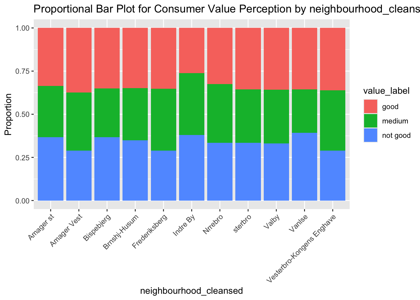
pro_chart_function('property_type')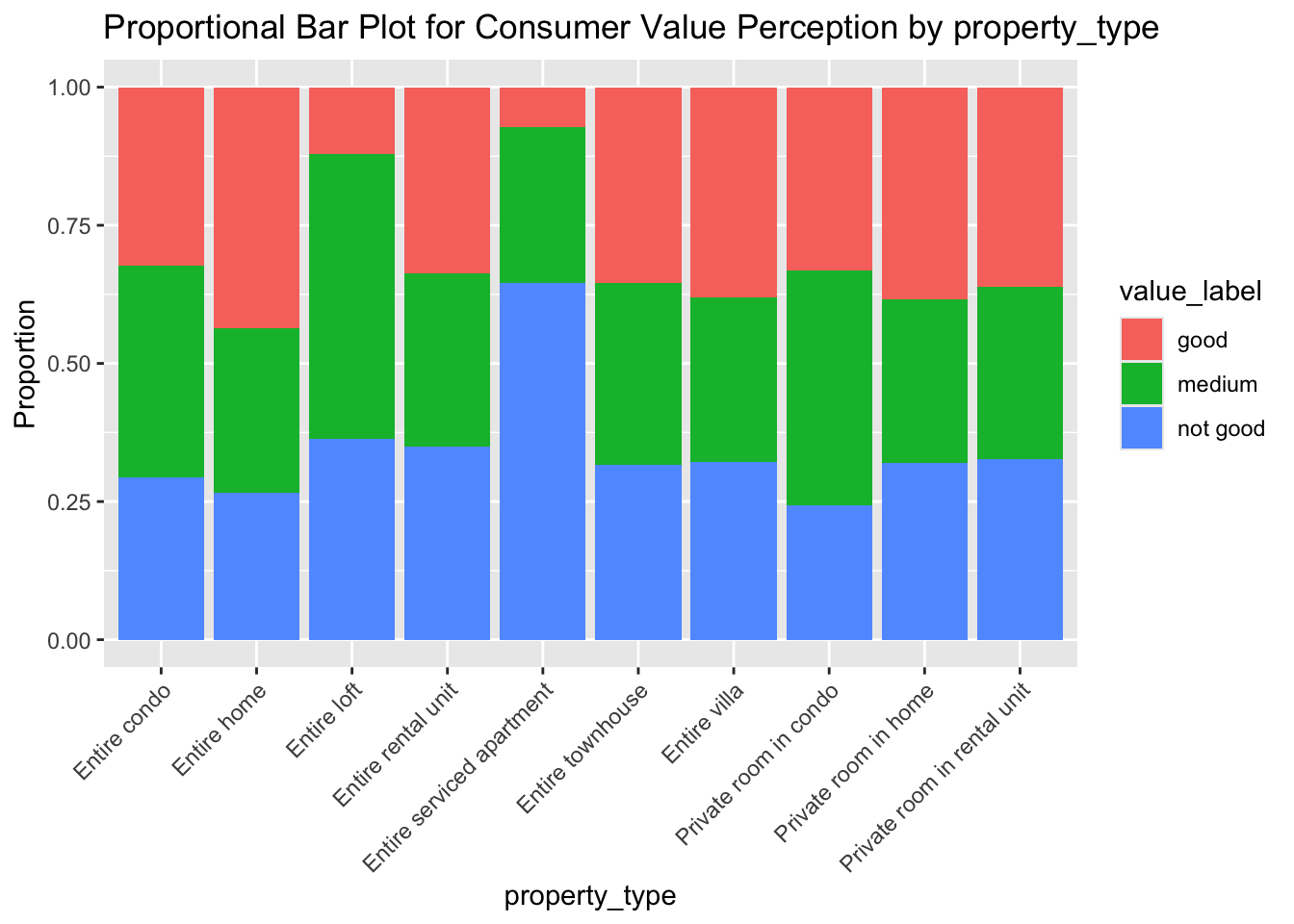
pro_chart_function('room_type')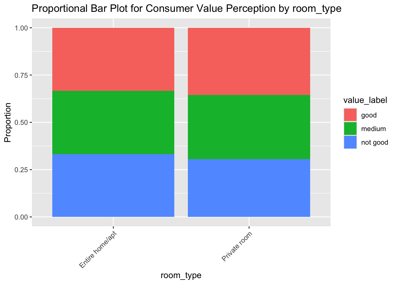
pro_chart_function('bathrooms_text')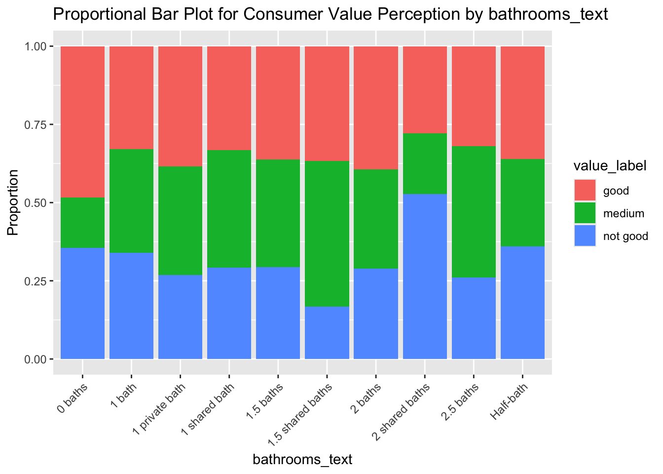
It seems that all of our input variables have some impact on the response variable (by showing results differences among different categories which are within the same input variables). For example, we can see that the Entire Serviced Apartment property type seems to be prone to generating customer reviews which are “not so good”. To assess the results in a more sophisticated way, we then build a naive bayes model:
# 5. Data Partitioning
set.seed(5)
train.index_naive = sample(c(1:nrow(naive_clean)),
                           nrow(naive_clean)*0.6)
train.set_naive = naive_clean[train.index_naive, ]
valid.set_naive = naive_clean[-train.index_naive, ]

# 6. Build the Naive Bayes Model
value.nb = naiveBayes(value_label ~ .,
                      data = train.set_naive,
                      laplace = 1) # Laplace (add-one) smoothing
value.nb
Naive Bayes Classifier for Discrete Predictors

Call:
naiveBayes.default(x = X, y = Y, laplace = laplace)

A-priori probabilities:
Y
     good    medium  not good
0.3377179 0.3304279 0.3318542

Conditional probabilities:
          neighbourhood_cleansed
Y           Amager st Amager Vest Bispebjerg Brnshj-Husum Frederiksberg
  good     0.07320507  0.09948381 0.04880338   0.01736274    0.11168466
  medium   0.07146283  0.09448441 0.03741007   0.01438849    0.11175060
  not good 0.08404967  0.07784145 0.05253104   0.01432665    0.10171920
          neighbourhood_cleansed
Y            Indre By    Nrrebro    sterbro      Valby     Vanlse
  good     0.13561708 0.16518067 0.10980760 0.03472548 0.02205537
  medium   0.17985612 0.17314149 0.09928058 0.03069544 0.01678657
  not good 0.18863419 0.17430755 0.10506208 0.03581662 0.02196753
          neighbourhood_cleansed
Y          Vesterbro-Kongens Enghave
  good                    0.18723604
  medium                  0.17601918
  not good                0.14899713

          property_type
Y          Entire condo Entire home Entire loft Entire rental unit
  good      0.243078367 0.054434538 0.002815580        0.580947912
  medium    0.292086331 0.037889688 0.011031175        0.534772182
  not good  0.232091691 0.037726839 0.007163324        0.603629417
          property_type
Y          Entire serviced apartment Entire townhouse Entire villa
  good                   0.003284843      0.024401689  0.010793055
  medium                 0.011510791      0.020143885  0.008153477
  not good               0.025310411      0.020057307  0.008595989
          property_type
Y          Private room in condo Private room in home
  good               0.017832004          0.008916002
  medium             0.025419664          0.008153477
  not good           0.013371538          0.009551098
          property_type
Y          Private room in rental unit
  good                     0.058188644
  medium                   0.055635492
  not good                 0.047277937

          room_type
Y          Entire home/apt Private room
  good          0.91694040   0.08399812
  medium        0.91270983   0.08824940
  not good      0.93170965   0.06924546

          bathrooms_text
Y              0 baths      1 bath 1 private bath 1 shared bath   1.5 baths
  good     0.004692633 0.794931957    0.011262318   0.051149695 0.058657907
  medium   0.002398082 0.799520384    0.014868106   0.060431655 0.058513189
  not good 0.002865330 0.833333333    0.008118434   0.041547278 0.049188157
          bathrooms_text
Y          1.5 shared baths     2 baths 2 shared baths   2.5 baths   Half-bath
  good          0.003284843 0.066635382    0.002815580 0.005631159 0.005631159
  medium        0.004796163 0.050359712    0.002398082 0.006235012 0.005275779
  not good      0.001910220 0.049665712    0.004775549 0.005253104 0.008118434
A fictional rental scenario we made up is located in Valby, is the entire home, and has 1.5 shared baths. Our model shows that the A-priori probabilities for the 3 target bins are 0.3374610 (good), 0.3334521 (medium) and 0.3290869 (not good), respectively. The model predicts that our fictional rental (which is in the neighborhood Valby, is the Entire Home property type, is the Entire home/apt room type, and has 1.5 shared baths) will be likely to receive “Good” reviews from customers.
# 7. Make a prediction based on a fictional rental scenario
fiction_rental = data.frame(
  neighbourhood_cleansed = 'Valby',
  property_type = 'Entire home',
  room_type = 'Entire home/apt',
  bathrooms_text = '1.5 shared baths'
)

fic.pred = predict(value.nb, fiction_rental)
fic.pred
[1] good
Levels: good medium not goodNext, we assessed our model using the validation set:
# 8. Assessing the model
train_pred = predict(value.nb, train.set_naive)
train_matrix = confusionMatrix(train_pred, train.set_naive$value_label)
train_accuracy = train_matrix$overall['Accuracy']
train_accuracy
Accuracy
0.3904913 train_matrixConfusion Matrix and Statistics
Reference
Prediction good medium not good
good 791 603 612
medium 608 750 559
not good 732 732 923
Overall Statistics
Accuracy : 0.3905
95% CI : (0.3784, 0.4027)
No Information Rate : 0.3377
P-Value [Acc > NIR] : < 2.2e-16
Kappa : 0.0858
Mcnemar's Test P-Value : 2.062e-07
Statistics by Class:
Class: good Class: medium Class: not good
Sensitivity 0.3712 0.3597 0.4408
Specificity 0.7093 0.7238 0.6528
Pos Pred Value 0.3943 0.3912 0.3867
Neg Pred Value 0.6887 0.6961 0.7015
Prevalence 0.3377 0.3304 0.3319
Detection Rate 0.1254 0.1189 0.1463
Detection Prevalence 0.3179 0.3038 0.3783
Balanced Accuracy 0.5402 0.5417 0.5468valid_pred = predict(value.nb, valid.set_naive)
valid_matrix = confusionMatrix(valid_pred, valid.set_naive$value_label)
valid_accuracy = valid_matrix$overall['Accuracy']
valid_accuracy Accuracy
0.3769011 valid_matrixConfusion Matrix and Statistics
Reference
Prediction good medium not good
good 490 466 416
medium 407 484 355
not good 498 480 612
Overall Statistics
Accuracy : 0.3769
95% CI : (0.3622, 0.3917)
No Information Rate : 0.3398
P-Value [Acc > NIR] : 2.564e-07
Kappa : 0.066
Mcnemar's Test P-Value : 1.343e-06
Statistics by Class:
Class: good Class: medium Class: not good
Sensitivity 0.3513 0.3385 0.4425
Specificity 0.6865 0.7257 0.6538
Pos Pred Value 0.3571 0.3884 0.3849
Neg Pred Value 0.6809 0.6806 0.7055
Prevalence 0.3315 0.3398 0.3287
Detection Rate 0.1164 0.1150 0.1454
Detection Prevalence 0.3260 0.2961 0.3779
Balanced Accuracy 0.5189 0.5321 0.5482The confusion matrices for the training set and validation set show that the respective accuracy scores are 0.3846 (train set) and 0.3749 (valid set). The similar accuracy scores demonstrate that there is no overfitting concern in our model. As for the naive method, as we have 3 classes which are binned by the equal frequency method, the naive rates for all 3 classes will be around 33.33% (100%/3). In other words, our model will have a 12.48% improvement (using the 37.49% accuracy rate of the validation set) compared to the naive method, proving the value of our naive bayes model.
In summary, to predict the review_scores_value which shows how much value a customer sees in the rental experience, our team used an equal frequency binning method which splits the target variable into 3 bins – good, medium, and not good. We built a naive bayes model which uses the neighbourhood_cleansed, property_type, room_type, bathrooms_text variables (all categorical) as input variables, because we infer that these rental features are most likely to make a difference in determining a customer’s perceived value gained. Note that for both the property_type and bathrooms_text variables, only the 10 most frequent values are kept to simplify our analysis. Our model predicts that a fictional rental which is in the neighborhood Valby, is the Entire Home property type, is the Entire home/apt room type, and has 1.5 shared baths will probably receive “Good” reviews from customers.
When assessing our model against both the training data and validation data, it has been found that the model’s accuracy is more than 37% in both cases. This means that we can get a 12.48% improvement compared to the naive method which predicts the probabilities to be 33.33% for all 3 bins. In other words, when taking values from the rental’s neighborhood, property, room and bathroom features, we are more confident than the naive method that we’ll predict customers’ value review types correctly.
Classification Tree
To predict whether a rental is short-term or long-term, we used a classification tree model with the following features: host_is_superhost, neighbourhood_cleansed, host_identity_verified, property_type, room_type, accommodates, bathrooms, bedrooms, price, review_scores_rating, has_availability.
library(rpart)
library(rpart.plot)
tree_data <- copenhagen %>%
select(host_is_superhost,
neighbourhood_cleansed,
host_identity_verified,
property_type,
room_type,
accommodates,
bathrooms,
bedrooms,
# beds,
price,
review_scores_rating,
has_availability,
minimum_nights)
sum(is.na(tree_data))[1] 0Since property_type had too many unique values, we restricted it to the top 10 most frequent property types.
top_10_property <- tree_data %>%
  count(property_type, sort = TRUE) %>%
  slice(1:10)

tree_data = tree_data %>%
  filter(property_type %in% top_10_property$property_type)

tree_data$host_identity_verified <- factor(tree_data$host_identity_verified)
tree_data$property_type <- factor(tree_data$property_type)
tree_data$neighbourhood_cleansed <- factor(tree_data$neighbourhood_cleansed)
tree_data$host_is_superhost <- factor(tree_data$host_is_superhost)
tree_data$has_availability <- factor(tree_data$has_availability)
After cleaning the data, we binned minimum_nights into 3 categories: short(<2 nights), medium(2-5 nights), and long (>5 nights). What’s interesting, at the beginning we tried to bin minimum_nights into 2 categories, but observed a large number of extremely long stays (e.g., >100 nights). Thus, using three categories provided a better balance between classes and more meaningful distinctions in rental behavior.
# Bin the minimum nights into 3 bins
tree_data$rental_type <- cut(tree_data$minimum_nights,
                             breaks = c(0, 2, 5, Inf),
                             labels = c("Short", "Medium", "Long"))
table(tree_data$rental_type)
 Short Medium   Long
  4661   4915   1001
tree_data <- tree_data %>% select(-minimum_nights)
summary(tree_data) host_is_superhost neighbourhood_cleansed host_identity_verified
FALSE:8690 Vesterbro-Kongens Enghave:1839 FALSE:1013
TRUE :1887 Indre By :1775 TRUE :9564
Nrrebro :1753
Frederiksberg :1122
sterbro :1102
Amager Vest : 948
(Other) :2038
property_type room_type accommodates
Entire rental unit :6055 Length:10577 Min. : 1.000
Entire condo :2681 Class :character 1st Qu.: 2.000
Private room in rental unit: 580 Mode :character Median : 3.000
Entire home : 481 Mean : 3.379
Entire townhouse : 213 3rd Qu.: 4.000
Private room in condo : 205 Max. :16.000
(Other) : 362
bathrooms bedrooms price review_scores_rating
Min. :0.000 Min. :0.000 Min. : 72 Min. :0.000
1st Qu.:1.000 1st Qu.:1.000 1st Qu.: 900 1st Qu.:4.750
Median :1.000 Median :1.000 Median : 1160 Median :4.910
Mean :1.096 Mean :1.604 Mean : 1365 Mean :4.831
3rd Qu.:1.000 3rd Qu.:2.000 3rd Qu.: 1600 3rd Qu.:5.000
Max. :5.000 Max. :8.000 Max. :20000 Max. :5.000
has_availability rental_type
FALSE: 1 Short :4661
TRUE :10576 Medium:4915
Long :1001
# data partitioning
set.seed(79)
tree_data.index <- sample(c(1:nrow(tree_data)), nrow(tree_data)*0.6)
train_set <- tree_data[tree_data.index, ]
valid_set <- tree_data[-tree_data.index, ]

tree_model <- rpart(rental_type ~ .,
                    method = 'class',
                    data = train_set)

rpart.plot(tree_model)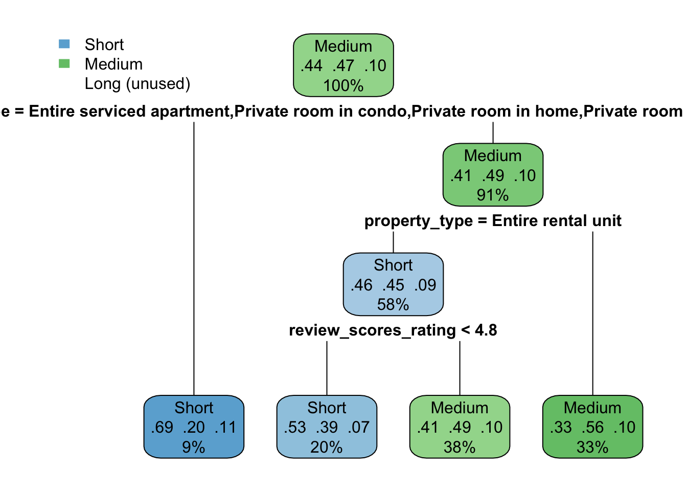
Our initial tree was very shallow (only one level) and did not perform well. We applied cross-validation to select optimal cp value that minimizes prediction error. After pruning the tree using optimal cp, the final tree performed better: the training set’s accuracy is 56.35%, while the validation set’s is 54.15%. While the overall accuracy is lower, the smaller performance gap between training and validation data indicates that the pruned tree generalizes better and is less prone to overfitting.
#cross validation
five_fold_cv <-
  rpart(rental_type ~ .,method = 'class', cp=0.00001, minsplit=5, xval=5,  data = train_set)
a <- printcp(five_fold_cv)
Classification tree:
rpart(formula = rental_type ~ ., data = train_set, method = "class",
    cp = 1e-05, minsplit = 5, xval = 5)

Variables actually used in tree construction:
[1] accommodates           bathrooms              bedrooms
[4] host_identity_verified host_is_superhost      neighbourhood_cleansed
[7] price                  property_type          review_scores_rating

Root node error: 3381/6346 = 0.53278

n= 6346

           CP nsplit rel error  xerror     xstd
1  8.3999e-02      0   1.00000 1.00000 0.011755
2  2.6028e-02      1   0.91600 0.91600 0.011777
3  4.4366e-03      3   0.86395 0.87578 0.011754
4  3.8450e-03      4   0.85951 0.88287 0.011760
5  2.3662e-03      6   0.85182 0.88169 0.011759
6  2.2183e-03     12   0.83614 0.87814 0.011756
7  2.0704e-03     14   0.83171 0.87844 0.011757
8  1.7746e-03     16   0.82757 0.89086 0.011766
9  1.4789e-03     19   0.82224 0.89796 0.011770
10 1.4131e-03     22   0.81781 0.89707 0.011769
11 1.3310e-03     31   0.80509 0.89737 0.011769
12 1.2817e-03     35   0.79976 0.89737 0.011769
13 1.1831e-03     40   0.79326 0.89825 0.011770
14 8.8731e-04     45   0.78734 0.89737 0.011769
15 8.0281e-04     86   0.73499 0.89737 0.011769
16 7.8872e-04     93   0.72937 0.90121 0.011772
17 7.6900e-04     97   0.72612 0.90121 0.011772
18 7.3943e-04    108   0.71251 0.90121 0.011772
19 6.9013e-04    118   0.70453 0.90565 0.011774
20 5.9154e-04    128   0.69713 0.91423 0.011777
21 5.3239e-04    186   0.66075 0.92754 0.011780
22 5.1760e-04    195   0.65513 0.92931 0.011780
23 5.0281e-04    216   0.64360 0.92990 0.011780
24 4.9295e-04    232   0.63472 0.92990 0.011780
25 4.7323e-04    256   0.62082 0.92931 0.011780
26 4.4366e-04    290   0.60367 0.92961 0.011780
27 3.9436e-04    340   0.58089 0.93286 0.011781
28 3.6971e-04    398   0.55546 0.93375 0.011781
29 3.5492e-04    408   0.55161 0.95327 0.011779
30 3.3274e-04    416   0.54865 0.95327 0.011779
31 2.9577e-04    426   0.54481 0.95652 0.011779
32 2.5880e-04    820   0.40994 0.96510 0.011776
33 2.4648e-04    840   0.40402 0.96510 0.011776
34 2.3662e-04    850   0.40106 0.96717 0.011775
35 2.3004e-04    877   0.39456 0.96717 0.011775
36 2.2183e-04    886   0.39249 0.96747 0.011775
37 1.9718e-04    925   0.38332 0.97338 0.011773
38 1.8486e-04   1008   0.36616 0.97338 0.011773
39 1.7746e-04   1018   0.36409 0.98344 0.011767
40 1.6901e-04   1028   0.36202 0.98344 0.011767
41 1.4789e-04   1048   0.35759 0.98492 0.011766
42 1.1831e-04   1138   0.34369 0.98521 0.011766
43 9.8590e-05   1145   0.34280 0.98906 0.011764
44 7.3943e-05   1172   0.34014 0.99024 0.011763
45 6.5727e-05   1176   0.33984 0.98994 0.011763
46 5.9154e-05   1185   0.33925 0.98994 0.011763
47 1.0000e-05   1195   0.33866 0.98994 0.011763
# Re-build model with optimal CP value
pruned.ct <- prune(five_fold_cv,
cp=five_fold_cv$cptable[which.min(five_fold_cv$cptable[,"xerror"]),"CP"])
rpart.plot(pruned.ct,type=5, extra = 2, fallen.leaves=FALSE)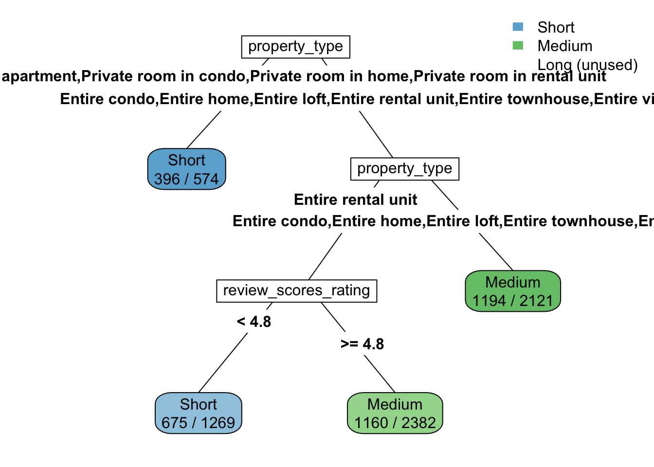
head(rpart.rules(pruned.ct)) rental_type Sho Med Lon
Short [.53 .39 .07] when property_type is Entire rental unit & review_scores_rating < 4.8
Short [.69 .20 .11] when property_type is Entire serviced apartment or Private room in condo or Private room in home or Private room in rental unit
Medium [.41 .49 .10] when property_type is Entire rental unit & review_scores_rating >= 4.8
Medium [.33 .56 .10] when property_type is Entire condo or Entire home or Entire loft or Entire townhouse or Entire villa #assessing model
# Training Set
train.pred <- predict(pruned.ct, train_set, type="class")
confusionMatrix(train.pred, train_set$rental_type)Confusion Matrix and Statistics
Reference
Prediction Short Medium Long
Short 1071 611 161
Medium 1693 2354 456
Long 0 0 0
Overall Statistics
Accuracy : 0.5397
95% CI : (0.5274, 0.552)
No Information Rate : 0.4672
P-Value [Acc > NIR] : < 2.2e-16
Kappa : 0.1507
Mcnemar's Test P-Value : < 2.2e-16
Statistics by Class:
Class: Short Class: Medium Class: Long
Sensitivity 0.3875 0.7939 0.00000
Specificity 0.7845 0.3644 1.00000
Pos Pred Value 0.5811 0.5228 NaN
Neg Pred Value 0.6240 0.6685 0.90277
Prevalence 0.4355 0.4672 0.09723
Detection Rate 0.1688 0.3709 0.00000
Detection Prevalence 0.2904 0.7096 0.00000
Balanced Accuracy 0.5860 0.5792 0.50000# Validation Set
valid.pred <- predict(pruned.ct, valid_set, type="class")
confusionMatrix(valid.pred, valid_set$rental_type)Confusion Matrix and Statistics
Reference
Prediction Short Medium Long
Short 704 416 91
Medium 1193 1534 293
Long 0 0 0
Overall Statistics
Accuracy : 0.529
95% CI : (0.5138, 0.5441)
No Information Rate : 0.4609
P-Value [Acc > NIR] : < 2.2e-16
Kappa : 0.132
Mcnemar's Test P-Value : < 2.2e-16
Statistics by Class:
Class: Short Class: Medium Class: Long
Sensitivity 0.3711 0.7867 0.00000
Specificity 0.7828 0.3485 1.00000
Pos Pred Value 0.5813 0.5079 NaN
Neg Pred Value 0.6050 0.6565 0.90924
Prevalence 0.4484 0.4609 0.09076
Detection Rate 0.1664 0.3626 0.00000
Detection Prevalence 0.2862 0.7138 0.00000
Balanced Accuracy 0.5769 0.5676 0.50000Property type, price, and number of bedrooms are among the most influential variables in predicting whether a rental is short-, medium-, or long-term. However, since the overall model performance is not so high, it suggests that rental duration is hard to predict based on listing features alone. Other factors — such as individual traveler preferences, trip purpose, or external events — likely play a major role in determining how long guests stay, but these factors are not captured in the dataset.
Clustering
To cluster properties we used 7 features and created new variable “price per bedroom”. The neighborhood_cleansed and room_type columns were listed as categorical variables, so we converted them to factors and assigned them dummy values, since k-means clustering requires all input features to be numeric.
# Select features
features <- copenhagen %>%
  select(price, number_of_reviews, review_scores_rating, minimum_nights, bedrooms,
         neighbourhood_cleansed, room_type)

#  Check NAs
colSums(is.na(features))
price number_of_reviews review_scores_rating
0 0 0
minimum_nights bedrooms neighbourhood_cleansed
0 0 0
room_type
0 # Create new feature: price_per_bedroom
features <- features %>%
mutate(price_per_bedroom = price / bedrooms)
features$price_per_bedroom[is.infinite(features$price_per_bedroom)] <- NA
features <- features %>% drop_na()
# Convert categorical columns to factors
features$neighbourhood_cleansed <- as.factor(features$neighbourhood_cleansed)
features$room_type <- as.factor(features$room_type)
# Create dummy variables
dummies <- dummyVars(~ neighbourhood_cleansed + room_type, data = features)
categorical_data <- as.data.frame(predict(dummies, newdata = features))
# Select numeric variables
numeric_data <- features %>%
select(price_per_bedroom, number_of_reviews, review_scores_rating, minimum_nights)Then, we combined our data together and scaled final data to ensure even weighting.
#  Combine data
final_data <- bind_cols(numeric_data, categorical_data)

# Scale the final dataset
scaled_data <- scale(final_data)

colSums(is.na(features))
price number_of_reviews review_scores_rating
0 0 0
minimum_nights bedrooms neighbourhood_cleansed
0 0 0
room_type price_per_bedroom
0 0 We then created an Elbow plot based on the scaled data to determine the ideal number of clusters. While the elbow plot is not a perfect way to determine the number of clusters (as there really is no perfect number) it can still give insight. We chose to use 3 clusters based on the elbow plot, and found three clusters resulted in distinguishable characteristics.
set.seed(9)
wss <- vector()

for (k in 1:10) {
  kmeans_model <- kmeans(scaled_data, centers = k, nstart = 25)
  wss[k] <- kmeans_model$tot.withinss
}

# Elbow plot
plot(1:10, wss, type = "b", pch = 19,
     xlab = "Number of Clusters (k)",
     ylab = "Total Within-Cluster Sum of Squares",
     main = "Elbow Method for Choosing k")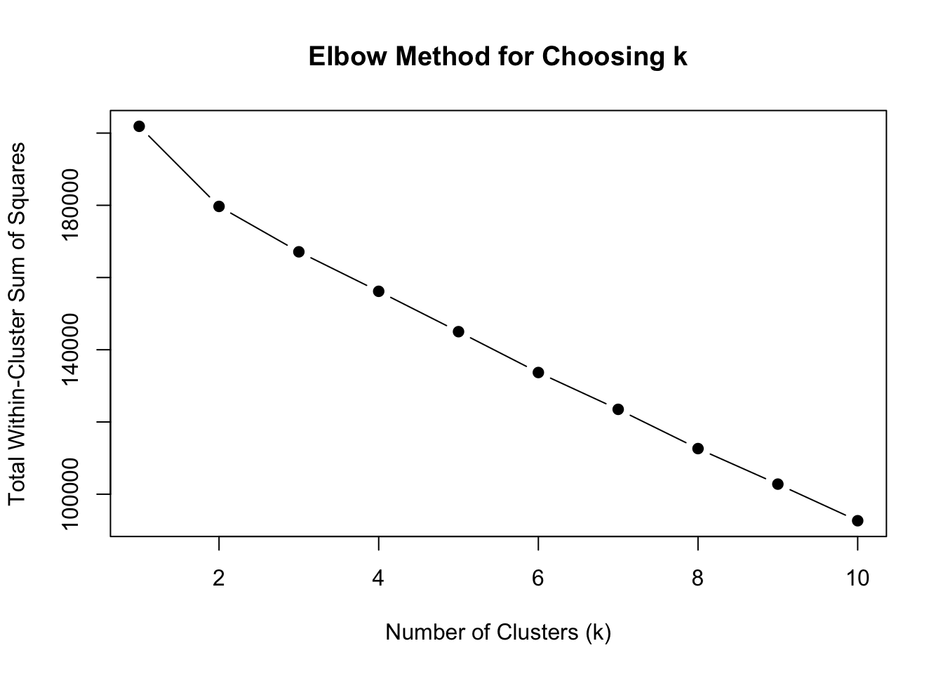
set.seed(9)
kmeans_model <- kmeans(scaled_data, centers = 3, nstart = 25)
features$cluster <- as.factor(kmeans_model$cluster)
As a result we have 3 Clusters:
Cluster 1: Apples - basic, common, and affordable; not many people’s favorite fruit but still solid. Lowest mean price per bedroom, highest mean number of reviews, smallest mean number of bedrooms, and slightly lower review scores. This indicates cheap, small properties that are popular but not necessarily top-rated.
Cluster 2: Mango - typically more expensive/seen as exotic, not everyone has tried it (medium # of reviews). Highest mean price per bedroom, medium number of reviews, and medium size. This may represent higher-end or luxury properties, potentially located in desirable neighborhoods but reviewed slightly less frequently.
Cluster 3: Strawberries - not as expensive as mangos but more expensive than apples, come in bunches like the bedrooms in these properties, and are many people’s favorite fruit. Medium mean price per bedroom, highest number of bedrooms, and highest review score. This suggests larger properties , offering excellent guest experiences at a moderate price.
# features
features %>%
  group_by(cluster) %>%
  summarise(across(everything(), list(mean = mean), .names = "mean_{col}"))
# A tibble: 3 × 9
cluster mean_price mean_number_of_reviews mean_review_scores_rating
<fct> <dbl> <dbl> <dbl>
1 1 632. 56.8 4.78
2 2 1701. 30.1 4.83
3 3 1295. 17.5 4.84
# ℹ 5 more variables: mean_minimum_nights <dbl>, mean_bedrooms <dbl>,
# mean_neighbourhood_cleansed <dbl>, mean_room_type <dbl>,
# mean_price_per_bedroom <dbl>ggplot(features, aes(x = cluster)) +
geom_bar(fill = "skyblue") +
geom_text(stat = "count", aes(label = ..count..), vjust = -0.5, size = 3) +
labs(title = "Number of Listings per Cluster",
x = "Cluster",
y = "Count of Listings") +
theme_minimal()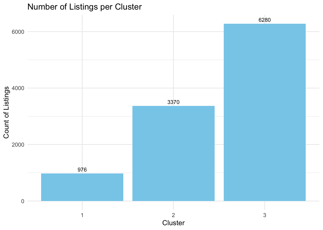
From first plot we see that, cluster 1 has 1890 values, cluster 2 has 6442, cluster 3 has 13214. Cluster 3 has a much higher amount of listings in it, suggesting the majority of listings are medium price, well reviewed, and have a greater number of bedrooms.
ggplot(features %>% filter(price < 10000),
       aes(x=room_type, y=price, fill=cluster)) +
  geom_bar(position="dodge", stat="identity") +
  labs(title = "Distribution of price within different room types per Cluster (price < 10000)",
       x = "Room Type",
       y = "Price") +
  theme_minimal()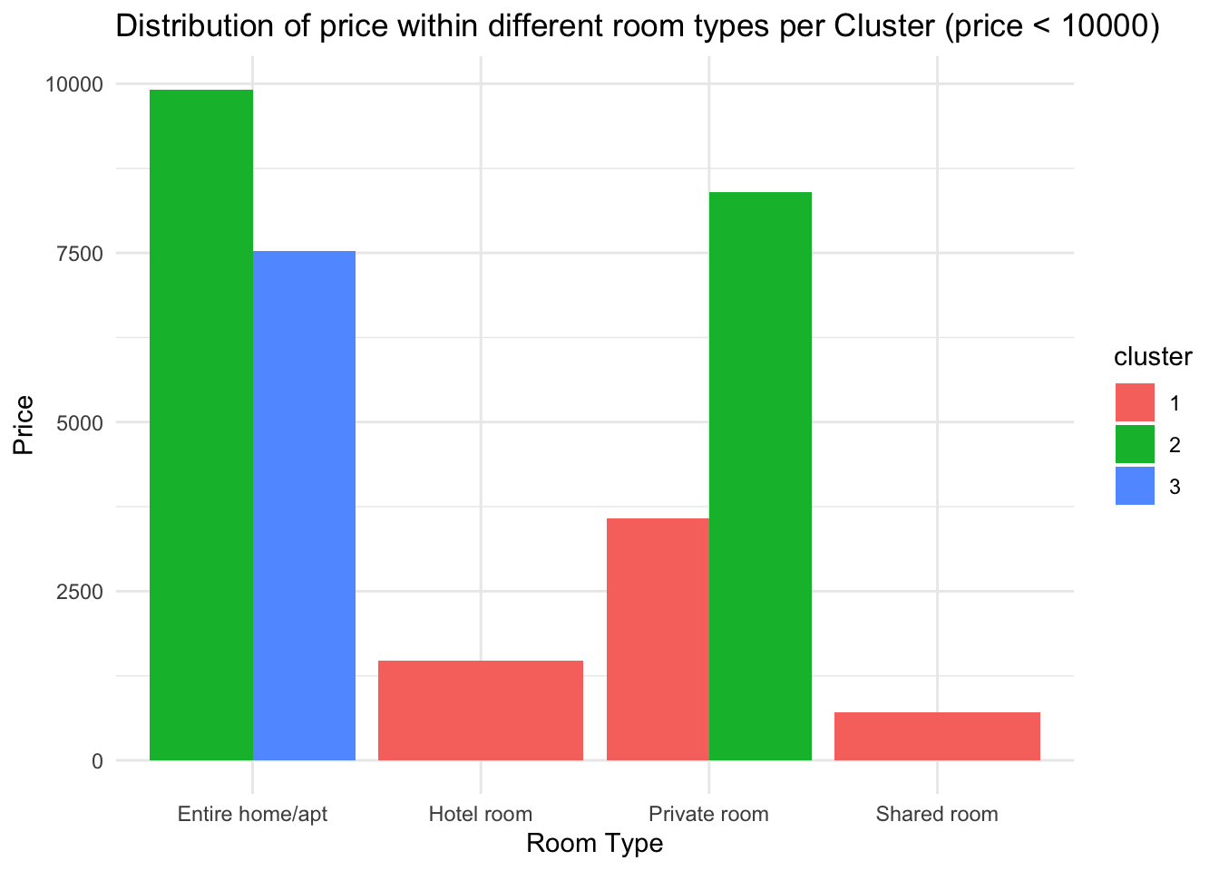
This plot shows the relationship between room type and price across clusters. We observe that Cluster 1 has the lowest prices, so it includes all kinds of room types . In contrast, Cluster 2 and Cluster 3 have much higher prices, and mainly offer entire homes/apartments. This suggests that higher-priced properties are usually entire listings, while lower-priced properties offer more diverse room options.
ggplot(features %>% filter(price < 5000),
       aes(x = price, y = review_scores_rating, color = cluster)) +
  geom_point(alpha = 0.7, size = 1.5) +
  scale_x_continuous(breaks = seq(0, 5000, by = 500)) +
  scale_y_continuous(breaks = seq(0, 5, by = 1)) +
  labs(
    title = "K-Means Clustering: Price per Bedroom vs Rating (price < 5000)",
    x = "Price per Bedroom",
    y = "Review Score Rating"
  ) +
  theme_minimal()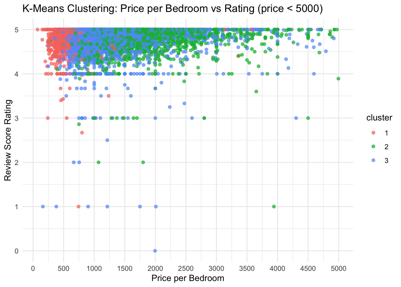
This plot shows that higher price per bedroom is not strongly associated with higher review scores. This suggests that customer satisfaction depends more on experience and value for money than on the property’s price. Thus, offering better service and cost performance is more important for achieving high ratings than simply charging more.
Conclusions
This project gave our team valuable hands-on experience in both technical and interpretive data mining. It was fascinating to learn about Copenhagen, a city which we had limited familiarity with, through the lens of the Airbnb rental market. Beyond the data itself, we gained insight into the geography, culture, and the tourism dynamics of Copenhagen. One of the biggest challenges we encountered was realizing that real-world data is rarely clean or complete. Throughout the project, we encountered missing values, inconsistent formats, and variables that did not always behave as expected. Through trial and error, data cleaning, and model adjustments, we were able to reach results we feel are meaningful and reflective of the Copenhagen rental market.
Some of the outcomes surprised us, while others were disappointing. The MLR, classification tree, regression, and naive bayes models reminded us that not every outcome is predictable in the real world, especially when human behavior is involved. This project proves that using more complicated methods does not necessarily lead to better predictions, and that in the real world any increase in accuracy, no matter how seemingly small, can be incredibly valuable. Real world data can also be shocking and questionable, listings priced over 60,000 DKK per night or minimum stays of over 200 nights could either represent exceptional cases or possible errors. What was ultimately most interesting about our work was seeing how different visualizations and modeling approaches revealed different parts of the same story. Rental markets are volatile, but certain themes consistently emerged across our analysis, like location and size importance to guests. This project reinforced the importance of patience and critical thinking when interpreting data. We must often look at the bigger picture and use domain knowledge to help understand the complexities of the real world.
The data mining findings from this project could be beneficial to a wide range of audiences, both within Copenhagen and beyond. In Copenhagen itself, the most obvious beneficiaries are Airbnb hosts themselves! These hosts could use the insights from our neighborhood trends, regression pricing model, and clustering analysis to better position their listings thus optimizing both demand and revenue. Understanding what characteristics drive guests to book a stay, leave a review, and pay a premium is incredibly valuable. Our cluster analysis allows hosts to better identify their direct competition and adjust their pricing and marketing strategies accordingly. Investors could use neighborhood analysis to identify more affordable neighborhoods for property acquisition or target higher value neighborhoods to increase profits. Similarly, travelers visiting Copenhagen on a specific budget can use the findings to select rental types and locations that best align with their needs and desires. Competitors such as hotels or Verbo hosts could also use the data to adapt their pricing models or service offerings based on Airbnb’s successes and shortcomings. Additionally, the Copenhagen tourism department could leverage the geographic patterns we uncovered to promote less-saturated neighborhoods and better understand the features of Copenhagen that are naturally attracting tourists. Existing Airbnb hosts could use our superhost analysis to strategically decide if pursuing superhost status would benefit their listings. Although our regression model indicated superhost is not a significant driver of pricing, neighborhood patterns showed where superhosts are concentrated. Achieving superhost status could be a way for hosts to differentiate in underrepresented neighborhoods and potentially boost bookings.
Outside of Copenhagen, city planners and analysts in other major urban cities could gain insights into what amenities, price points, and property types travelers prefer. Our modeling techniques, particularly the regression model and clustering analysis, could be replicated using other cities’ datasets to better understand their own local rental markets. Identifying which property features drive price premiums or rental satisfactions could help shape tourism strategies and investment decisions in cities with similar rental markets. Finally, marketers across the travel, real estate, and hospitality sectors would find significant value in this data mining work. Airbnb hosts, hotel brands, real estate agents, and tourism boards could all use our insights to better tailor their marketing strategies. In particular, our word cloud and clustering could help marketers craft more effective messaging by emulating key neighborhood descriptors and property features that are successful with Copenhagens’ guests. Popular property types, frequently mentioned listing characteristics, and pricing strategies identified in our analysis provide guidance for designing compelling marketing and promotional campaigns.
Our insight into which factors most influence pricing, listing successes, and guest satisfaction, our findings offer actionable strategies for a wide variety of audiences, both within Copenhagen and across the broader travel and hospitality industries.