library(tidyverse)
library(dplyr)
library(caret)
library(ggplot2)
library(e1071)

cc <- read.csv('consumer_complaints.csv')Complaint Classifier
As part of my Data Mining coursework, I’m building a Naive Bayes classification model to predict whether a consumer disputes a company’s response using the Consumer Complaints dataset. The project involves cleaning and preprocessing the data, including renaming variables, removing redundancies, and binning categories. I evaluate the model’s performance using confusion matrices and compare it to the naive rule, uncovering key insights into the challenges of predicting dispute outcomes and how predictions can be improved.
The source of dataset is Kaggle.
Data Exploration
Numeric: Resolution.time.in.days, Year
Categorical: X.ID
glimpse(cc)Rows: 14,000
Columns: 16
$ X.ID <int> 1615767, 654223, 1143398, 1303679, 1627370, 1…
$ Company <chr> "PHH Mortgage", "Ocwen", "Southwest Credit Sy…
$ Product <chr> "Mortgage", "Mortgage", "Debt collection", "C…
$ Issue <chr> "Loan servicing, payments, escrow account", "…
$ State <chr> "FL", "NC", "MO", "WA", "VA", "IL", "FL", "OK…
$ Submitted.via <chr> "Web", "Web", "Web", "Web", "Web", "Web", "We…
$ Date.received <chr> "10/20/2015", "3/1/2014", "4/12/2014", "03/26…
$ Date.resolved <chr> "10/20/2015", "3/1/2014", "4/12/2014", "03/26…
$ Timely.response. <chr> "Yes", "Yes", "Yes", "Yes", "Yes", "Yes", "Ye…
$ Consumer.disputed. <chr> "No", "No", "No", "No", "No", "No", "No", "No…
$ state.name <chr> "Florida", "North Carolina", "Missouri", "Was…
$ Date.received.1 <chr> "10/20/2015", "1/3/2014", "12/4/2014", "3/26/…
$ Date.resolved.1 <chr> "10/20/2015", "1/3/2014", "12/4/2014", "3/26/…
$ Resolution.time.in.days. <int> 0, 0, 0, 0, 0, 0, 1, 0, 0, 0, 5, 0, 0, 29, 0,…
$ Year <int> 2015, 2014, 2014, 2015, 2015, 2015, 2016, 201…
$ QTR..US.FLY. <chr> "Q4", "Q1", "Q4", "Q1", "Q4", "Q2", "Q2", "Q2…Consumer.disputed. variable is of type chr, then I converted it to factor. Now it has 2 levels: Yes or No.
We see that the data is imbalanced, out of 14,000 complaints only 3138 (22.4%) disputed.
str(cc$Consumer.disputed.) chr [1:14000] "No" "No" "No" "No" "No" "No" "No" "No" "No" "No" "No" "No" ...cc$Consumer.disputed. <- factor(cc$Consumer.disputed.)
levels(cc$Consumer.disputed.)[1] "No" "Yes"table(cc$Consumer.disputed.)
   No   Yes
10862  3138
cc %>% group_by(Consumer.disputed.) %>%
summarise(Count = n()/14000)# A tibble: 2 × 2
Consumer.disputed. Count
<fct> <dbl>
1 No 0.776
2 Yes 0.224I removed dots from variables that had them at the end, and renamed QTR..US.FLY. to Quarter.
names(cc) [1] "X.ID" "Company"
[3] "Product" "Issue"
[5] "State" "Submitted.via"
[7] "Date.received" "Date.resolved"
[9] "Timely.response." "Consumer.disputed."
[11] "state.name" "Date.received.1"
[13] "Date.resolved.1" "Resolution.time.in.days."
[15] "Year" "QTR..US.FLY." cc <- cc %>% rename(Resolution.time.in.days = Resolution.time.in.days.,
Timely.response=Timely.response.,
Consumer.disputed=Consumer.disputed.,
Quarter = QTR..US.FLY.)After examining number of unique values in each column, we observe that a few columns contain more than 100 distinct values. Specifically, there are 14,000 unique ID records, 1,050 companies, and over 1,300 date values.
sapply(cc, function(x) length(unique(x))) X.ID Company Product
14000 1050 12
Issue State Submitted.via
81 60 5
Date.received Date.resolved Timely.response
1370 1322 2
Consumer.disputed state.name Date.received.1
2 52 1370
Date.resolved.1 Resolution.time.in.days Year
1322 77 4
Quarter
4 cc <- cc %>% select(-X.ID, -Company, -Date.received, -Date.resolved, -Date.received.1, -Date.resolved.1)
str(cc)'data.frame': 14000 obs. of 10 variables:
$ Product : chr "Mortgage" "Mortgage" "Debt collection" "Credit card" ...
$ Issue : chr "Loan servicing, payments, escrow account" "Loan servicing, payments, escrow account" "Loan modification,collection,foreclosure" "Billing statement" ...
$ State : chr "FL" "NC" "MO" "WA" ...
$ Submitted.via : chr "Web" "Web" "Web" "Web" ...
$ Timely.response : chr "Yes" "Yes" "Yes" "Yes" ...
$ Consumer.disputed : Factor w/ 2 levels "No","Yes": 1 1 1 1 1 1 1 1 1 1 ...
$ state.name : chr "Florida" "North Carolina" "Missouri" "Washington" ...
$ Resolution.time.in.days: int 0 0 0 0 0 0 1 0 0 0 ...
$ Year : int 2015 2014 2014 2015 2015 2015 2016 2015 2013 2016 ...
$ Quarter : chr "Q4" "Q1" "Q4" "Q1" ...By examining the results of the summary() function, we notice an impossible negative number for the resolution date. Additionally, there are two overlapping columns: State and State_name.
summary(cc) Product Issue State Submitted.via
Length:14000 Length:14000 Length:14000 Length:14000
Class :character Class :character Class :character Class :character
Mode :character Mode :character Mode :character Mode :character
Timely.response Consumer.disputed state.name
Length:14000 No :10862 Length:14000
Class :character Yes: 3138 Class :character
Mode :character Mode :character
Resolution.time.in.days Year Quarter
Min. : -1.000 Min. :2013 Length:14000
1st Qu.: 0.000 1st Qu.:2014 Class :character
Median : 0.000 Median :2015 Mode :character
Mean : 2.006 Mean :2015
3rd Qu.: 2.000 3rd Qu.:2016
Max. :286.000 Max. :2016 Before that, when counting unique values by column, we observed that the State column had 60 unique values, while the State_name column had 52. Upon examining the values, it appears that the State column includes more detailed information, possibly encompassing territories and military postal codes. We can also keep Year, Resolution.time.in.days, and Quarter, which are related to the removed columns date_received, and date_resolved.
table(cc$State)
       AA   AE   AK   AL   AP   AR   AS   AZ   CA   CO   CT   DC   DE   FL   GA
 110    1    5   19  135    4   62    1  313 1977  251  161   98   80 1255  577
  GU   HI   IA   ID   IL   IN   KS   KY   LA   MA   MD   ME   MI   MN   MO   MP
   1   39   56   51  500  137   78   99  149  292  408   47  373  174  171    1
  MS   MT   NC   ND   NE   NH   NJ   NM   NV   NY   OH   OK   OR   PA   PR   RI
  77   19  443    7   54   65  518   75  171  996  463   93  177  511   26   64
  SC   SD   TN   TX   UT   VA   VI   VT   WA   WI   WV   WY
 194   26  238 1040   77  480    8   29  303  178   32   11
cc <- cc %>% select(-state.name) %>%
filter(Resolution.time.in.days>=0)
str(cc)'data.frame': 13997 obs. of 9 variables:
$ Product : chr "Mortgage" "Mortgage" "Debt collection" "Credit card" ...
$ Issue : chr "Loan servicing, payments, escrow account" "Loan servicing, payments, escrow account" "Loan modification,collection,foreclosure" "Billing statement" ...
$ State : chr "FL" "NC" "MO" "WA" ...
$ Submitted.via : chr "Web" "Web" "Web" "Web" ...
$ Timely.response : chr "Yes" "Yes" "Yes" "Yes" ...
$ Consumer.disputed : Factor w/ 2 levels "No","Yes": 1 1 1 1 1 1 1 1 1 1 ...
$ Resolution.time.in.days: int 0 0 0 0 0 0 1 0 0 0 ...
$ Year : int 2015 2014 2014 2015 2015 2015 2016 2015 2013 2016 ...
$ Quarter : chr "Q4" "Q1" "Q4" "Q1" ...The Year column contains four unique values: 2013, 2014, 2015, and 2016. For binning, we can group them into two categories: ‘Earlier period’ for 2013 and 2014, and ‘Later period’ for 2015 and 2016.
cc <- cc %>%
  mutate(Year = cut(Year,
                    breaks = c(2012, 2014, 2016),
                    labels = c("Earlier period", "Later period"),
                    right = TRUE))

str(cc)
'data.frame': 13997 obs. of 9 variables:
$ Product : chr "Mortgage" "Mortgage" "Debt collection" "Credit card" ...
$ Issue : chr "Loan servicing, payments, escrow account" "Loan servicing, payments, escrow account" "Loan modification,collection,foreclosure" "Billing statement" ...
$ State : chr "FL" "NC" "MO" "WA" ...
$ Submitted.via : chr "Web" "Web" "Web" "Web" ...
$ Timely.response : chr "Yes" "Yes" "Yes" "Yes" ...
$ Consumer.disputed : Factor w/ 2 levels "No","Yes": 1 1 1 1 1 1 1 1 1 1 ...
$ Resolution.time.in.days: int 0 0 0 0 0 0 1 0 0 0 ...
$ Year : Factor w/ 2 levels "Earlier period",..: 2 1 1 2 2 2 2 2 1 2 ...
$ Quarter : chr "Q4" "Q1" "Q4" "Q1" ...The Resolution_time variable contains a significant number of zeros (8,316) along with other values. This imbalance caused issues when using the equal frequency method for binning. To address this, I first filtered out the non-zero values to determine the breaks within the data. Then, I added zero to this group.
As a result, we have three groups: low, medium, and high.
table(cc$Resolution.time.in.days)
   0    1    2    3    4    5    6    7    8    9   10   11   12   13   14   15
8316 1616 1122  844  491  473  318  222   83   35   47   37   21   18   18   18
  16   17   18   19   20   21   22   23   24   25   26   27   28   29   30   31
   9   10   16   15   12   22    9    6   13    6    7    2   10   16    5    9
  32   33   34   35   36   37   38   39   40   41   42   43   45   46   47   48
  14    9    9   11   12    3    3    7    3    8    3    8    5    2    5    1
  49   50   51   52   55   56   57   60   61   63   64   65   66   67   68   70
   5    3    3    1    6    2    1    2    4    2    1    2    1    1    1    1
  72   76   77   79   83   90   93   95   98  106  151  286
   1    1    1    1    1    1    1    1    1    1    1    1
non_zero_values <- cc$Resolution.time.in.days[cc$Resolution.time.in.days > 0]
breaks <- quantile(non_zero_values, probs = seq(0, 1, length.out = 3))
breaks <- c(0, breaks)
cc$Resolution.time.in.days <- cut(cc$Resolution.time.in.days, breaks = breaks, labels = c("low", "medium", "high"), include.lowest = TRUE)
table(cc$Resolution.time.in.days)
   low medium   high
  9932   1966   2099
For the next few steps, we are going to be reducing the number of unique levels for some of our factor variables:
The Product column has 12 unique values, but we will use only the 6 most common ones.
length(unique(cc$Product))[1] 12top_6_Product <- cc %>%
count(Product, sort = TRUE) %>%
slice(1:6) %>%
select(Product)The Issue column contains 81 unique values, and we will use only the 7 most common ones. Also changed these 7 values to the shorter names.
length(unique(cc$Issue))[1] 81top_7_Issue <- cc %>%
count(Issue, sort = TRUE) %>%
slice(1:7) %>%
select(Issue)The State column has 60 unique values, and we will use the 10 most common ones.
length(unique(cc$State))[1] 60top_10_State <- cc %>%
count(State, sort = TRUE) %>%
slice(1:10) %>%
select(State)cc <- cc %>% filter(Product %in% top_6_Product$Product &
Issue %in% top_7_Issue$Issue &
State %in% top_10_State$State)
cc <- cc %>%
mutate(Issue = case_when(
Issue == "Account opening, closing, or management" ~ "Account Management",
Issue == "Application, originator, mortgage broker" ~ "Mortgage Application",
Issue == "Communication tactics" ~ "Communication",
Issue == "Credit reporting company's investigation" ~ "Credit Investigation",
Issue == "Deposits and withdrawals" ~ "Transactions",
Issue == "Loan modification,collection,foreclosure" ~ "Loan Modification",
Issue == "Loan servicing, payments, escrow account" ~ "Loan Servicing",
TRUE ~ Issue
))
nrow(cc)[1] 4110After reducing the unique levels, the dataset now contains 4110 rows.
str(cc)'data.frame': 4110 obs. of 9 variables:
$ Product : chr "Mortgage" "Mortgage" "Credit reporting" "Debt collection" ...
$ Issue : chr "Loan Servicing" "Mortgage Application" "Credit Investigation" "Loan Modification" ...
$ State : chr "FL" "FL" "CA" "NY" ...
$ Submitted.via : chr "Web" "Web" "Web" "Email" ...
$ Timely.response : chr "Yes" "Yes" "Yes" "Yes" ...
$ Consumer.disputed : Factor w/ 2 levels "No","Yes": 1 1 1 2 1 1 1 1 1 2 ...
$ Resolution.time.in.days: Factor w/ 3 levels "low","medium",..: 1 1 1 1 1 3 3 1 3 1 ...
$ Year : Factor w/ 2 levels "Earlier period",..: 2 2 2 1 2 1 2 2 2 1 ...
$ Quarter : chr "Q4" "Q2" "Q1" "Q4" ...cc$Product <- as.factor(cc$Product)
cc$Issue <- as.factor(cc$Issue)
cc$State <- as.factor(cc$State)
cc$Submitted.via <- as.factor(cc$Submitted.via)
cc$Timely.response <- as.factor(cc$Timely.response)
cc$Year <- as.factor(cc$Year)
cc$Quarter <- as.factor(cc$Quarter)Data Partitioning
After converting all variables to factor type, I partitioned the data into training(60%) and validation(40%) sets.
set.seed(79)
cc.index <- sample(c(1:nrow(cc)), nrow(cc)*0.6)
cc_train.df <- cc[cc.index, ]
cc_valid.df <- cc[-cc.index, ]
Data Visualization - Proportional Barplot
ggplot(cc_train.df, aes(x = Product, fill = Consumer.disputed)) +
    geom_bar(position = 'fill') +
  labs(x = "Product", y = "Proportion")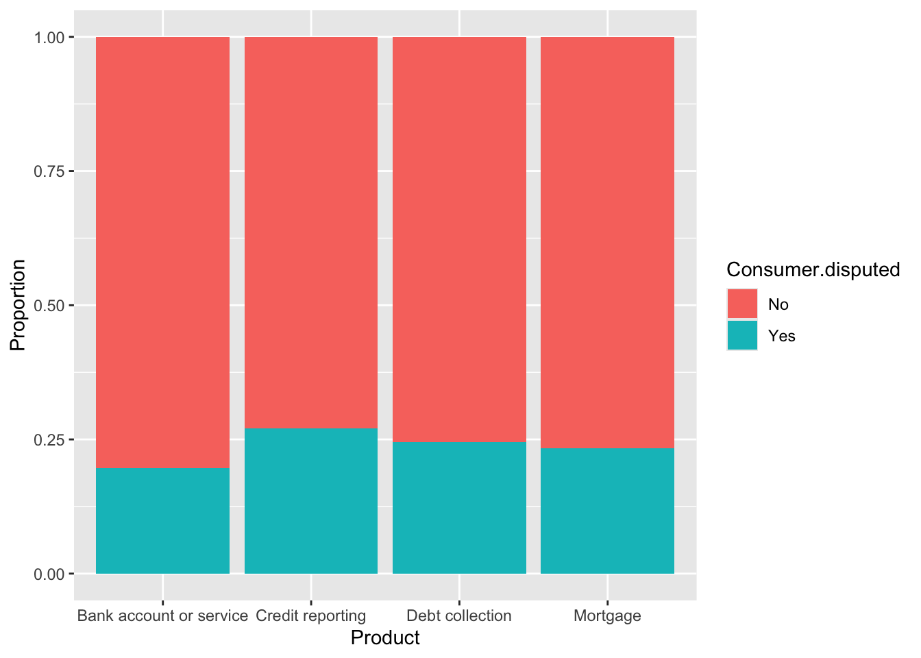
ggplot(cc_train.df, aes(x = Issue, fill = Consumer.disputed)) +
    geom_bar(position = 'fill') +
  # coord_flip() +
  theme(axis.text.x = element_text(angle = 45, hjust = 1)) +
  labs(x = "Issue", y = "Proportion")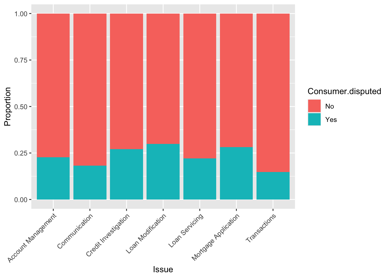
ggplot(cc_train.df, aes(x = State, fill = Consumer.disputed)) +
    geom_bar(position = 'fill') +
  labs(x = "State", y = "Proportion")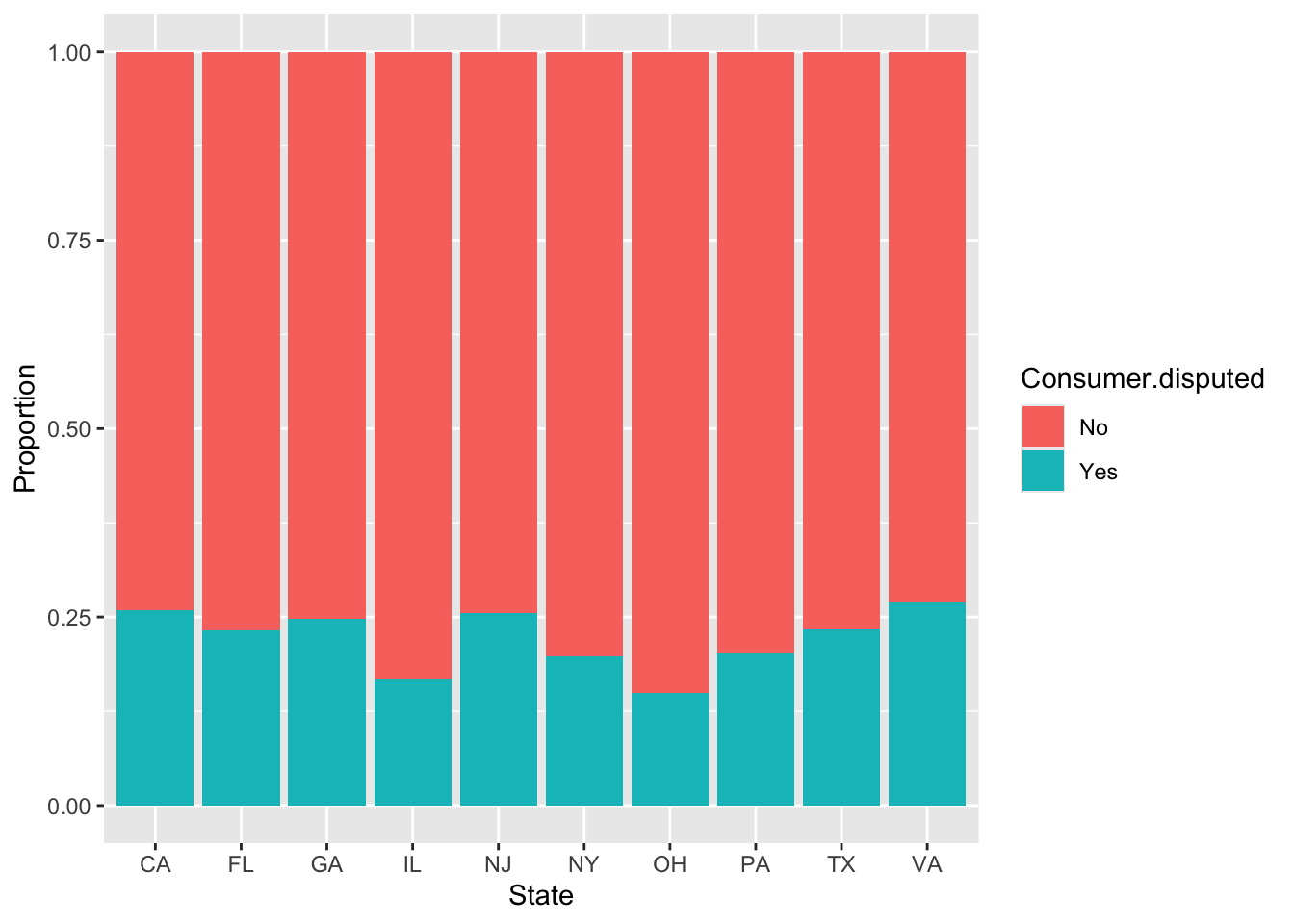
ggplot(cc_train.df, aes(x = Submitted.via, fill = Consumer.disputed)) +
    geom_bar(position = 'fill') +
  labs(x = "Submitted.via", y = "Proportion")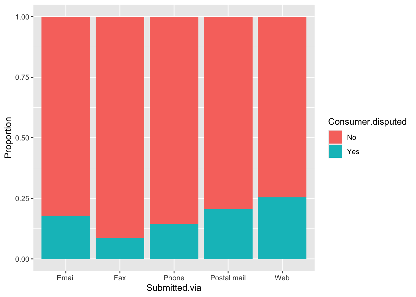
ggplot(cc_train.df, aes(x = Timely.response, fill = Consumer.disputed)) +
    geom_bar(position = 'fill') +
  labs(x = "Timely.response", y = "Proportion")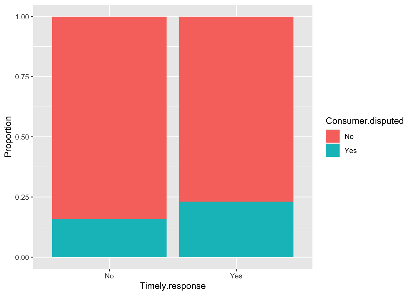
ggplot(cc_train.df, aes(x = Year, fill = Consumer.disputed)) +
    geom_bar(position = 'fill') +
  labs(x = "Year", y = "Proportion")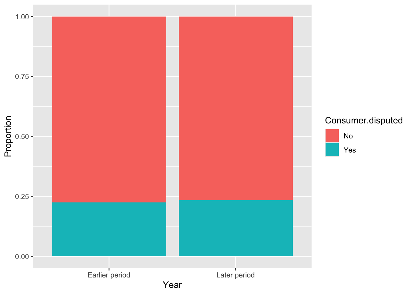
ggplot(cc_train.df, aes(x = Quarter, fill = Consumer.disputed)) +
    geom_bar(position = 'fill') +
  labs(x = "Quarter", y = "Proportion")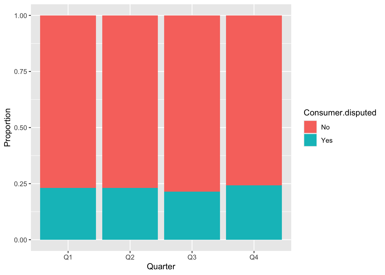
ggplot(cc_train.df, aes(x = Resolution.time.in.days, fill = Consumer.disputed)) +
    geom_bar(position = 'fill') +
  labs(x = "Resolution.time.in.days", y = "Proportion")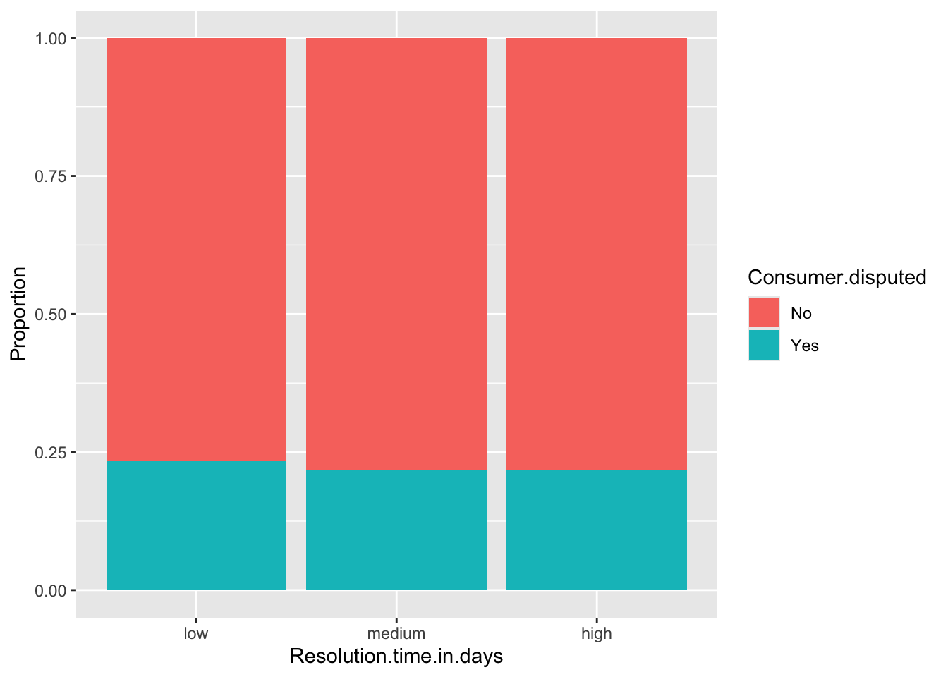
For the Year variable, we observed a similar proportion between time periods and whether consumers disputed or not. The same applies to the Quarter variable, with only a small difference in the third quarter. Timely.response showed better result with noticeable differences between values compared to Resolution.time.in.days. For the remaining variables, we can see distinct differences between categories.
I will remove Resolution.time.in.days, because of the imbalance of values in dataset.
cc_train.df <- cc_train.df %>% select(-Year, -Quarter, -Resolution.time.in.days)
str(cc_train.df)
'data.frame': 2466 obs. of 6 variables:
$ Product : Factor w/ 4 levels "Bank account or service",..: 3 1 4 3 4 3 1 3 3 4 ...
$ Issue : Factor w/ 7 levels "Account Management",..: 2 1 5 4 5 4 1 2 2 5 ...
$ State : Factor w/ 10 levels "CA","FL","GA",..: 2 5 2 8 8 5 4 3 9 1 ...
$ Submitted.via : Factor w/ 5 levels "Email","Fax",..: 5 5 5 4 5 4 1 5 5 5 ...
$ Timely.response : Factor w/ 2 levels "No","Yes": 2 2 2 2 2 2 2 2 2 2 ...
$ Consumer.disputed: Factor w/ 2 levels "No","Yes": 1 1 1 2 1 1 1 1 1 1 ...cc.nb <- naiveBayes(Consumer.disputed ~.,data = cc_train.df)
cc.nb
Naive Bayes Classifier for Discrete Predictors

Call:
naiveBayes.default(x = X, y = Y, laplace = laplace)

A-priori probabilities:
Y
       No       Yes
0.7704785 0.2295215

Conditional probabilities:
     Product
Y     Bank account or service Credit reporting Debt collection   Mortgage
  No               0.27210526       0.08368421      0.22473684 0.41947368
  Yes              0.22261484       0.10424028      0.24558304 0.42756184

     Issue
Y     Account Management Communication Credit Investigation Loan Modification
  No          0.15947368    0.11105263           0.08368421        0.11368421
  Yes         0.15724382    0.08303887           0.10424028        0.16254417
     Issue
Y     Loan Servicing Mortgage Application Transactions
  No      0.34421053           0.07526316   0.11263158
  Yes     0.32862191           0.09893993   0.06537102

     State
Y             CA         FL         GA         IL         NJ         NY
  No  0.22578947 0.15631579 0.07210526 0.06526316 0.06000000 0.11789474
  Yes 0.26501767 0.15901060 0.07950530 0.04416961 0.06890459 0.09717314
     State
Y             OH         PA         TX         VA
  No  0.06000000 0.06000000 0.12736842 0.05526316
  Yes 0.03533569 0.05123675 0.13074205 0.06890459

     Submitted.via
Y           Email         Fax       Phone Postal mail         Web
  No  0.176315789 0.011052632 0.089473684 0.042631579 0.680526316
  Yes 0.128975265 0.003533569 0.051236749 0.037102473 0.779151943

     Timely.response
Y             No        Yes
  No  0.01684211 0.98315789
Yes 0.01060071 0.98939929str(cc_train.df)'data.frame': 2466 obs. of 6 variables:
$ Product : Factor w/ 4 levels "Bank account or service",..: 3 1 4 3 4 3 1 3 3 4 ...
$ Issue : Factor w/ 7 levels "Account Management",..: 2 1 5 4 5 4 1 2 2 5 ...
$ State : Factor w/ 10 levels "CA","FL","GA",..: 2 5 2 8 8 5 4 3 9 1 ...
$ Submitted.via : Factor w/ 5 levels "Email","Fax",..: 5 5 5 4 5 4 1 5 5 5 ...
$ Timely.response : Factor w/ 2 levels "No","Yes": 2 2 2 2 2 2 2 2 2 2 ...
$ Consumer.disputed: Factor w/ 2 levels "No","Yes": 1 1 1 2 1 1 1 1 1 1 ...Confusion Matrix
Comparing the accuracy metrics, the validation set achieved 74.45%, which is lower than the training set’s 77.05%. However, both sets reveal that the model predominantly predicts ‘No’ for all instances (100%). a.The model predicts ‘No’ for every case and never predicts ‘Yes’, indicating an imbalance among predictions. Although the accuracy appears relatively high, it is misleading as it reflects the model’s bias rather than its true predictive power.
confusionMatrix(predict(cc.nb, newdata=cc_train.df), cc_train.df$Consumer.disputed)Confusion Matrix and Statistics
Reference
Prediction No Yes
No 1900 566
Yes 0 0
Accuracy : 0.7705
95% CI : (0.7534, 0.7869)
No Information Rate : 0.7705
P-Value [Acc > NIR] : 0.5113
Kappa : 0
Mcnemar's Test P-Value : <2e-16
Sensitivity : 1.0000
Specificity : 0.0000
Pos Pred Value : 0.7705
Neg Pred Value : NaN
Prevalence : 0.7705
Detection Rate : 0.7705
Detection Prevalence : 1.0000
Balanced Accuracy : 0.5000
'Positive' Class : No
confusionMatrix(predict(cc.nb, newdata=cc_valid.df), cc_valid.df$Consumer.disputed)Confusion Matrix and Statistics
Reference
Prediction No Yes
No 1224 420
Yes 0 0
Accuracy : 0.7445
95% CI : (0.7227, 0.7655)
No Information Rate : 0.7445
P-Value [Acc > NIR] : 0.5131
Kappa : 0
Mcnemar's Test P-Value : <2e-16
Sensitivity : 1.0000
Specificity : 0.0000
Pos Pred Value : 0.7445
Neg Pred Value : NaN
Prevalence : 0.7445
Detection Rate : 0.7445
Detection Prevalence : 1.0000
Balanced Accuracy : 0.5000
'Positive' Class : No
Naive Rule vs Naive Bayes
Naive rule in classification is to classify the record as a member of majority class. If we had used the naive rule for classification, we would classify all records in the training set as “No” because “No” is the most frequent class.
Our Naive Bayes model, which follows the naive rule approach, assigns all cases as “No.” Both methods yield the same accuracy of 77.05%, resulting in a 0% difference between them.
I think imbalance plays a big role here. As described in the book, the absence of this predictor actively “outvotes” any other information in the record to assign a “No” to the outcome value (when, in this case, it has a relatively good chance of being a “Yes”). Also, as a customer, I often choose not to dispute issues to avoid wasting energy. It’s usually easier to let things go rather than engage in disputes, especially if the potential outcome doesn’t seem worth the effort. Maybe it’s a reason why we don’t have meaningful data.
Scoring data using Naive Bayes
I took 25 records by sorting the probability for the “Yes” column in descending order, selecting the top 25 as the most likely to belong to the “YES” group.
Among these 25 records, 5 records truly belong to “Yes” group. The accuracy for these predictions = 80%. Even though the model didn’t predict any “Yes” values, it still achieved 80% accuracy by correctly classifying 20 out of 20 “No” records. Since the “Yes” group is a small portion of the dataset, its impact on accuracy is minimal. Compared to accuracy of overall model 74.45%, these selected proportion of data have relatively high value.
pred.prob <- predict(cc.nb, newdata=cc_valid.df, type="raw")
# pred.prob

pred.class <- predict(cc.nb, newdata=cc_valid.df)
# pred.class

df <- data.frame(actual=cc_valid.df$Consumer.disputed,
                 predicted=pred.class, pred.prob)

valid_25 <- df %>% arrange(desc(Yes)) %>% slice(1:25)

table(valid_25$actual)
 No Yes
 20   5
valid_25 %>% filter(actual == 'Yes') actual predicted No Yes
1 Yes No 0.5992883 0.4007117
2 Yes No 0.6009522 0.3990478
3 Yes No 0.6009522 0.3990478
4 Yes No 0.6137075 0.3862925
5 Yes No 0.6137075 0.3862925Identifying this subset of records helps us to see that the model completely fails at identifying “Yes” cases. On the other hand, by assigning all records to the majority class “No,” the model achieves high accuracy, performing well in most cases. By identifying this main issue, we can focus on other ways to dealing with imbalanced data or try other models.
Manual calculation of probability
my_data <- cc_train.df[45,]
my_data
Product Issue State Submitted.via Timely.response
3560 Mortgage Mortgage Application IL Web No
Consumer.disputed
3560 Nopredict(cc.nb, my_data)[1] No
Levels: No Yespredict(cc.nb, my_data, type="raw") No Yes
[1,] 0.8370455 0.1629545cc.nb
Naive Bayes Classifier for Discrete Predictors

Call:
naiveBayes.default(x = X, y = Y, laplace = laplace)

A-priori probabilities:
Y
       No       Yes
0.7704785 0.2295215

Conditional probabilities:
     Product
Y     Bank account or service Credit reporting Debt collection   Mortgage
  No               0.27210526       0.08368421      0.22473684 0.41947368
  Yes              0.22261484       0.10424028      0.24558304 0.42756184

     Issue
Y     Account Management Communication Credit Investigation Loan Modification
  No          0.15947368    0.11105263           0.08368421        0.11368421
  Yes         0.15724382    0.08303887           0.10424028        0.16254417
     Issue
Y     Loan Servicing Mortgage Application Transactions
  No      0.34421053           0.07526316   0.11263158
  Yes     0.32862191           0.09893993   0.06537102

     State
Y             CA         FL         GA         IL         NJ         NY
  No  0.22578947 0.15631579 0.07210526 0.06526316 0.06000000 0.11789474
  Yes 0.26501767 0.15901060 0.07950530 0.04416961 0.06890459 0.09717314
     State
Y             OH         PA         TX         VA
  No  0.06000000 0.06000000 0.12736842 0.05526316
  Yes 0.03533569 0.05123675 0.13074205 0.06890459

     Submitted.via
Y           Email         Fax       Phone Postal mail         Web
  No  0.176315789 0.011052632 0.089473684 0.042631579 0.680526316
  Yes 0.128975265 0.003533569 0.051236749 0.037102473 0.779151943

     Timely.response
Y             No        Yes
  No  0.01684211 0.98315789
  Yes 0.01060071 0.98939929
no_score <- 0.7704785 * 0.41947368 * 0.07526316 * 0.06526316 * 0.680526316 * 0.01684211
yes_score <- 0.2295215 * 0.42756184 * 0.09893993 * 0.04416961 * 0.779151943 * 0.01060071
no_score/(no_score + yes_score)[1] 0.8370455I selected 45th row from training set.
- Actual Consumer.disputed outcome is “No”
- The model’s predicted answer is “No”
- The probability for “No” is 0.8370455, “Yes” is 0.1629545.