library(tidyverse)
library(dplyr)
library(arules)
library(arulesViz)

data("Groceries")Association rules
For this task, we will be using data from Groceries, a dataset that can be found with the arules package. Each row in the file represents one buyer’s purchases. We will generate item frequency plots, identify strong association rules involving a specific product, and visualize rules using scatter and graph-based methods.
This work is part of an assignment for the AD699 Data Mining course.
Groceries is of class transactions (sparse matrix). The data consists of 9835 rows, and 169 columns.
summary(Groceries)transactions as itemMatrix in sparse format with
9835 rows (elements/itemsets/transactions) and
169 columns (items) and a density of 0.02609146
most frequent items:
whole milk other vegetables rolls/buns soda
2513 1903 1809 1715
yogurt (Other)
1372 34055
element (itemset/transaction) length distribution:
sizes
1 2 3 4 5 6 7 8 9 10 11 12 13 14 15 16
2159 1643 1299 1005 855 645 545 438 350 246 182 117 78 77 55 46
17 18 19 20 21 22 23 24 26 27 28 29 32
29 14 14 9 11 4 6 1 1 1 1 3 1
Min. 1st Qu. Median Mean 3rd Qu. Max.
1.000 2.000 3.000 4.409 6.000 32.000
includes extended item information - examples:
labels level2 level1
1 frankfurter sausage meat and sausage
2 sausage sausage meat and sausage
3 liver loaf sausage meat and sausageThe bar plot below displays frequent items, that meet the support value. The minimum support threshold is set at 7.25%, meaning that only items appearing in at least 7.25% of all transactions are considered frequent. As a result we got 16 frequent products.
itemFrequencyPlot(Groceries,
                  support=0.0725,
                  horiz = TRUE,
                  col = "ivory",
                  main = "Frequent Grocery items (Support > 7.25%)")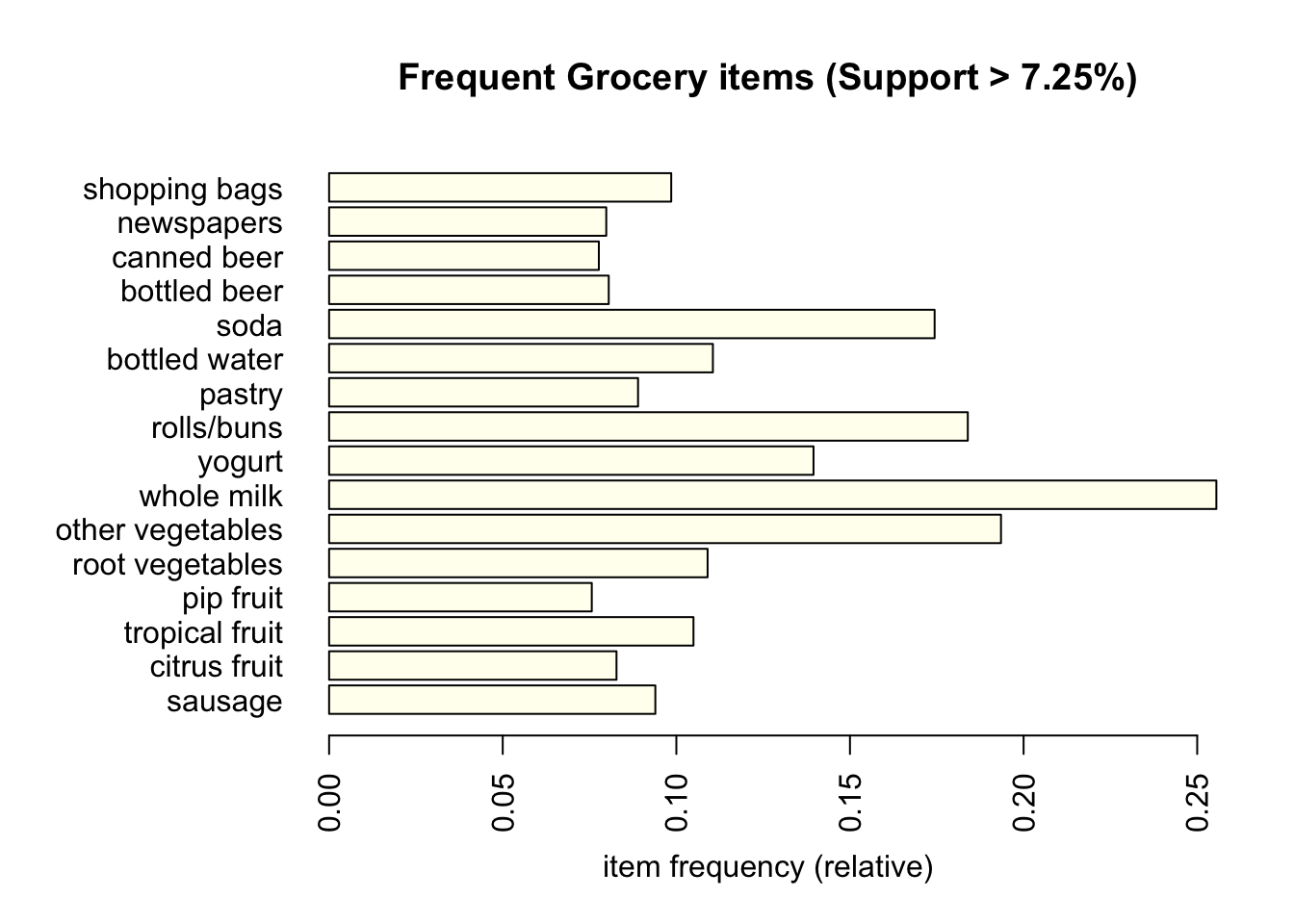
Let’s create subset of rules that contain my grocery item - cream cheese.
rules <- apriori (Groceries, parameter = list(supp = 0.001, conf = 0.5))Apriori
Parameter specification:
confidence minval smax arem aval originalSupport maxtime support minlen
0.5 0.1 1 none FALSE TRUE 5 0.001 1
maxlen target ext
10 rules TRUE
Algorithmic control:
filter tree heap memopt load sort verbose
0.1 TRUE TRUE FALSE TRUE 2 TRUE
Absolute minimum support count: 9
set item appearances ...[0 item(s)] done [0.00s].
set transactions ...[169 item(s), 9835 transaction(s)] done [0.00s].
sorting and recoding items ... [157 item(s)] done [0.00s].
creating transaction tree ... done [0.00s].
checking subsets of size 1 2 3 4 5 6 done [0.01s].
writing ... [5668 rule(s)] done [0.00s].
creating S4 object ... done [0.00s].# summary(rules)
# inspect(rules[1:5])
# itemLabels(Groceries)
lhs_rules <- subset(rules, lhs %in% "cream cheese ")
rhs_rules <- subset(rules, rhs %in% "cream cheese ")
summary(lhs_rules)set of 233 rules
rule length distribution (lhs + rhs):sizes
3 4 5
59 137 37
Min. 1st Qu. Median Mean 3rd Qu. Max.
3.000 3.000 4.000 3.906 4.000 5.000
summary of quality measures:
support confidence coverage lift
Min. :0.001017 Min. :0.5000 Min. :0.001118 Min. : 1.957
1st Qu.:0.001118 1st Qu.:0.5556 1st Qu.:0.001729 1st Qu.: 2.642
Median :0.001220 Median :0.6154 Median :0.002034 Median : 3.138
Mean :0.001536 Mean :0.6480 Mean :0.002494 Mean : 3.563
3rd Qu.:0.001729 3rd Qu.:0.7143 3rd Qu.:0.002847 3rd Qu.: 3.982
Max. :0.006609 Max. :1.0000 Max. :0.012405 Max. :11.041
count
Min. :10.00
1st Qu.:11.00
Median :12.00
Mean :15.11
3rd Qu.:17.00
Max. :65.00
mining info:
data ntransactions support confidence
Groceries 9835 0.001 0.5
call
apriori(data = Groceries, parameter = list(supp = 0.001, conf = 0.5))summary(rhs_rules)set of 1 rules
rule length distribution (lhs + rhs):sizes
5
1
Min. 1st Qu. Median Mean 3rd Qu. Max.
5 5 5 5 5 5
summary of quality measures:
support confidence coverage lift
Min. :0.001017 Min. :0.5882 Min. :0.001729 Min. :14.83
1st Qu.:0.001017 1st Qu.:0.5882 1st Qu.:0.001729 1st Qu.:14.83
Median :0.001017 Median :0.5882 Median :0.001729 Median :14.83
Mean :0.001017 Mean :0.5882 Mean :0.001729 Mean :14.83
3rd Qu.:0.001017 3rd Qu.:0.5882 3rd Qu.:0.001729 3rd Qu.:14.83
Max. :0.001017 Max. :0.5882 Max. :0.001729 Max. :14.83
count
Min. :10
1st Qu.:10
Median :10
Mean :10
3rd Qu.:10
Max. :10
mining info:
data ntransactions support confidence
Groceries 9835 0.001 0.5
call
apriori(data = Groceries, parameter = list(supp = 0.001, conf = 0.5))There is 233 rules that contain my product - on the left hand side. 59 rules involve three product subset, 137 four product subset, and 37 five product subset. And we get only 1 rule with cream cheese on right hand side, which is in the subset of five products. Indicating that cream cheese appears in combination with other products.
Let’s look at the first rule: If a person buys other vegetables, curd, yogurt, and whipped/sour cream this person 14.83 times more likely to buy cream cheese than a random customer in store. The support number is 0.001, meaning that 0.1% of all transactions studied had exact same item sets. Confidence is 0.59 => If someone buys other vegetables, curd, yogurt, and whipped/sour cream, there’s a 59% chance that they also buy cream cheese. Coverage number gives an idea how often the rule can be applied, in this case it equals to 0.002. This rule applies to 0.2% of all transactions in the dataset.
inspect(sort(rhs_rules, by="lift")) lhs rhs support confidence coverage lift count
[1] {other vegetables,
curd,
yogurt,
whipped/sour cream} => {cream cheese } 0.001016777 0.5882353 0.001728521 14.83409 10The next rule: If a person buys citrus fruit, other vegetables, whole milk, and cream cheese he/she is 9.12 times more likely to buy domestic eggs than a random purchaser in store. The support number is 0.001, this rule applies to only 0.1% of all transactions. This rule also have high confidence, saying that if customer buys citrus fruit, other vegetables, whole milk, and cream cheese, there is 58% chance they also buy domestic eggs. Coverage number is 0.002, meaning that this combination occurs in 0.2% of all transactions.
inspect(sort(lhs_rules, by="lift")[2]) lhs rhs support confidence coverage lift count
[1] {citrus fruit,
other vegetables,
whole milk,
cream cheese } => {domestic eggs} 0.001118454 0.5789474 0.001931876 9.124916 11From these rules we see that certain sets of products are frequently purchased together. In combination they may be ingredients for salads, or other recipes. Cream cheese, in particular, is commonly used in baking and is a key ingredient in cheesecake. Despite that, cream cheese widely used for frosting, spreads, pasta sauces, dips, making it a versatile ingredient in a variety of dishes.
By identifying frequent combinations with cream cheese, the store can strategically place those items nearby—such as positioning cream cheese close to the vegetables/fruits section or within the dairy aisle for convenient access. Also, offering special discounts can boost sales. For example, if a customer buys cream cheese, offering a discount on berries or bagels can encourage bundled purchases. Additionally, analyzing product pairs allows the store to anticipate demand and adjust inventory accordingly, ensuring high-demand combinations are well-stocked ahead of time, especially during peak shopping seasons.
inspect(lhs_rules[7:9]) lhs rhs support confidence
[1] {cream cheese , frozen meals} => {whole milk} 0.001016777 0.7142857
[2] {hard cheese, cream cheese } => {other vegetables} 0.001118454 0.5789474
[3] {hard cheese, cream cheese } => {whole milk} 0.001016777 0.5263158
coverage lift count
[1] 0.001423488 2.795464 10
[2] 0.001931876 2.992090 11
[3] 0.001931876 2.059815 10 plot(lhs_rules[7:9])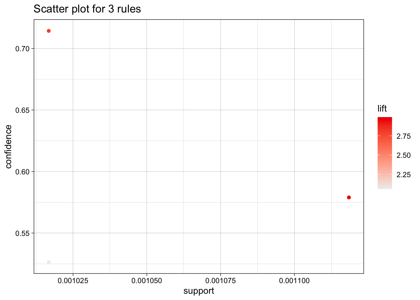
From the plot above, we observe the distribution of three association rules based on confidence (y-axis), support (x-axis), and lift (represented by color). First rule: {cream cheese , frozen meals} => {whole milk} has the highest confidence and lift values but a low support. This means the rule highly reliable: there is 71.43% chance that a customer who buys cream cheese and frozen meals will also buy whole milk. And the strength of the association is strong. However, it applies to 0.10% of the transactions. Second rule: {hard cheese, cream cheese } => {other vegetables} has a higher support and lift compared to the first rule, but its confidence is lower (57.9%). This suggests that while this combination of products occurs more frequently, it may not be as strong in predicting the purchase of vegetables when a customer buys both hard cheese and cream cheese. Third rule: {hard cheese, cream cheese } => {whole milk} has a similar support as a first rule, meaning that it applies to the same small proportion of transactions. However, it has lowest confidence and lift values, making it less reliable and significant to customer behaviour. This rule can demonstrate rare combination of items.
plot(lhs_rules[7:9], method = "graph", engine="htmlwidget")Now the plot shows the relationship between rules as a graph. The central node represents cream cheese, which appears in all three rules, indicating that it is a key item in these associations. Hard cheese and whole milk appear in two rules each, showing that these items are associated with more than one combination of products. Frozen meals and other vegetables only appear in one rule each, which indicates that they are more specific to particular product combinations. Also the color differentiation in the plot corresponds to the lift value of each rule. The rule 3, which has lowest lift value in represented in light red. Meanwhile, Rules 1 and 2 are highlighted in bold red, suggesting that they have higher lift values and stronger associations between the items. Compared to previous plot, this visual shows elements of rules, allowing to quickly identify the central elements, and the relative strength of the rules. This plot also displays measures of rules (confidence, support) if we click on rule node. However, if we want to select strong rule the scatter plot is more useful because it clearly shows rules with higher support and confidence in a more clearer way. Therefore, the choice of plot depends on the purpose.