Forecasting the salaries of hockey players

This project focuses on forecasting hockey player salaries by utilizing statistical analysis and machine learning methods. By analyzing player performance metrics, historical salary information, and other relevant factors, the project aims to deliver precise salary predictions.

This work is part of an assignment for the AD699 Data Mining course.

Simple Linear Regression

library(tidyverse)
library(dplyr)
library(ggplot2)
library(forecast)
library(gplots)

main_data <- read.csv('nhl_players.csv')

By looking at dataset, we can see that all variables that are represented by number are numeric. Even the salary column is represented as character because of the dollar sign, it is also numeric. And all other remaining variables are categorical.

Categorical: name, Team_y, Position_y, Handed
Numeric: GP, G, A, P, Sh, Sh_perc, Salary, PIM, Giveaways, Takeaways, Hits, Hits.Taken, blocked_shots, PlusMinus

Discrete numeric: GP, G, A, P, Sh, Giveaways, Takeaways, Hits, Hits.Taken, blocked_shots, PlusMinus Continuous numeric: Sh_perc, Salary, PIM

glimpse(main_data)

Rows: 568
Columns: 18
$ name          <chr> "Zemgus Girgensons", "Zack Smith", "Zack Kassian", "Zach…
$ Team_y        <chr> "BUF", "CHI", "EDM", "MIN", "TOR", "BUF, T.B", "BUF, T.B…
$ Position_y    <chr> "C", "C", "W", "W", "W", "D", "D", "C", "C", "W", "C", "…
$ HANDED        <chr> "Left", "Left", "Right", "Left", "Right", "Right", "Righ…
$ GP            <int> 68, 50, 59, 69, 51, 27, 27, 57, 70, 68, 63, 70, 55, 68, …
$ G             <int> 12, 4, 15, 25, 21, 1, 1, 6, 10, 31, 15, 7, 4, 8, 17, 1, …
$ A             <int> 7, 7, 19, 21, 16, 6, 6, 7, 20, 28, 31, 12, 17, 17, 14, 7…
$ P             <int> 19, 11, 34, 46, 37, 7, 7, 13, 30, 59, 46, 19, 21, 25, 31…
$ Sh            <int> 85, 43, 99, 155, 106, 29, 29, 98, 110, 197, 138, 99, 62,…
$ Sh_perc       <dbl> 0.14, 0.09, 0.15, 0.16, 0.20, 0.03, 0.03, 0.06, 0.09, 0.…
$ SALARY        <chr> "$1,600,000", "$3,250,000", "$2,000,000", "$9,000,000", …
$ PIM           <int> 10, 29, 69, 8, 23, 22, 22, 28, 49, 12, 16, 39, 6, 66, 45…
$ Giveaways     <int> 11, 14, 45, 22, 16, 11, 11, 21, 14, 41, 37, 8, 27, 18, 2…
$ Takeaways     <int> 13, 21, 26, 21, 32, 4, 4, 20, 48, 42, 54, 22, 10, 27, 25…
$ Hits          <int> 110, 112, 157, 27, 52, 30, 30, 136, 78, 9, 40, 213, 31, …
$ Hits.Taken    <int> 71, 71, 54, 60, 101, 21, 21, 99, 114, 66, 94, 129, 54, 6…
$ blocked_shots <int> 20, 18, 8, 38, 23, 27, 27, 30, 20, 14, 38, 11, 75, 29, 4…
$ PlusMinus     <int> -1, 2, 0, -11, 13, 0, 0, 6, -5, -2, 11, 0, -8, -21, -5, …

Our dataset doesn’t have any NA values.

colSums(is.na(main_data))

         name        Team_y    Position_y        HANDED            GP 
            0             0             0             0             0 
            G             A             P            Sh       Sh_perc 
            0             0             0             0             0 
       SALARY           PIM     Giveaways     Takeaways          Hits 
            0             0             0             0             0 
   Hits.Taken blocked_shots     PlusMinus 
            0             0             0 

I renamed the columns ‘Team_y’, ‘Position_y’ by removing last two characters, since they are not useful at all.

main_data <- main_data %>% rename(Team = Team_y, Position = Position_y)
names(main_data)

 [1] "name"          "Team"          "Position"      "HANDED"       
 [5] "GP"            "G"             "A"             "P"            
 [9] "Sh"            "Sh_perc"       "SALARY"        "PIM"          
[13] "Giveaways"     "Takeaways"     "Hits"          "Hits.Taken"   
[17] "blocked_shots" "PlusMinus"    

There are 7 duplicated name values found, after removing them we had 561 values in dataset.

main_data$name[duplicated(main_data$name)]

[1] "Zach Bogosian"     "Valeri Nichushkin" "Troy Brouwer"     
[4] "Paul Byron"        "Kevin Shattenkirk" "Corey Perry"      
[7] "Andrej Sekera"    

clean_data <- main_data %>% distinct(name, .keep_all = TRUE)
nrow(clean_data)

[1] 561

After clearing up the Salary variable from specific characters, I converted it to numeric type.

clean_data$SALARY <- as.numeric(gsub("[$,]", "", clean_data$SALARY))
str(clean_data)

'data.frame':   561 obs. of  18 variables:
 $ name         : chr  "Zemgus Girgensons" "Zack Smith" "Zack Kassian" "Zach Parise" ...
 $ Team         : chr  "BUF" "CHI" "EDM" "MIN" ...
 $ Position     : chr  "C" "C" "W" "W" ...
 $ HANDED       : chr  "Left" "Left" "Right" "Left" ...
 $ GP           : int  68 50 59 69 51 27 57 70 68 63 ...
 $ G            : int  12 4 15 25 21 1 6 10 31 15 ...
 $ A            : int  7 7 19 21 16 6 7 20 28 31 ...
 $ P            : int  19 11 34 46 37 7 13 30 59 46 ...
 $ Sh           : int  85 43 99 155 106 29 98 110 197 138 ...
 $ Sh_perc      : num  0.14 0.09 0.15 0.16 0.2 0.03 0.06 0.09 0.16 0.11 ...
 $ SALARY       : num  1600000 3250000 2000000 9000000 2500000 6000000 1000000 6300000 9000000 5900000 ...
 $ PIM          : int  10 29 69 8 23 22 28 49 12 16 ...
 $ Giveaways    : int  11 14 45 22 16 11 21 14 41 37 ...
 $ Takeaways    : int  13 21 26 21 32 4 20 48 42 54 ...
 $ Hits         : int  110 112 157 27 52 30 136 78 9 40 ...
 $ Hits.Taken   : int  71 71 54 60 101 21 99 114 66 94 ...
 $ blocked_shots: int  20 18 8 38 23 27 30 20 14 38 ...
 $ PlusMinus    : int  -1 2 0 -11 13 0 6 -5 -2 11 ...

Data partitioning helps prevent biased decisions by ensuring that insights from training dataset also applicable to validation set. If we analyze first, we may unintentionally use insights that we think are applicable for every scenario while it can lead to overfitting. By partitioning first, we can ensure that our tests on training and validation sets provide independent performance measures.

set.seed(79)
nhl.index <- sample(c(1:nrow(clean_data)), nrow(clean_data)*0.6)
nhl_train.df <- clean_data[nhl.index, ]
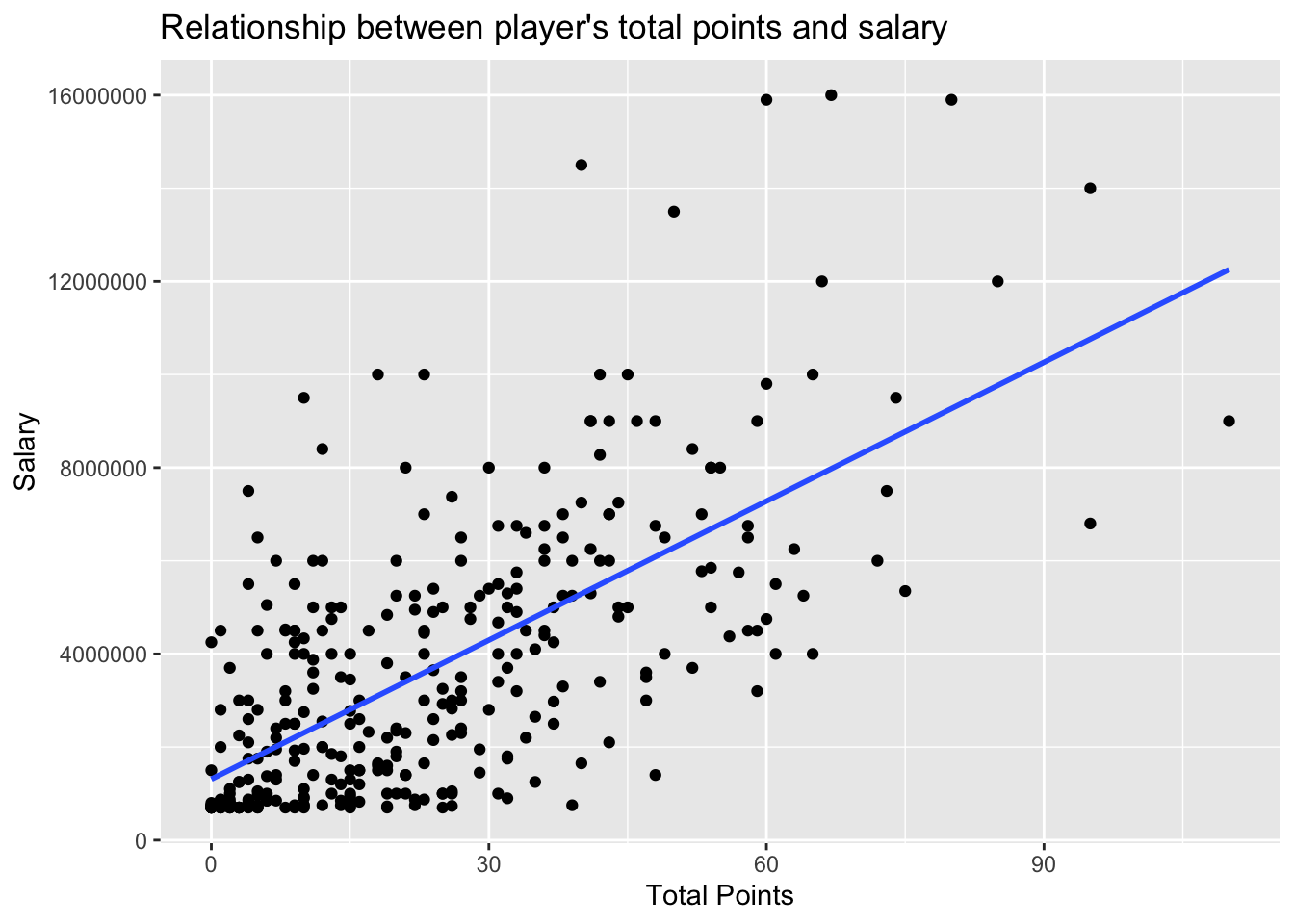
nhl_valid.df <- clean_data[-nhl.index, ]

From the plot below we can see that most of players with small salary also have small number of points, and by increase of total points salary also going up. However despite the total points, it seems like other parameters also affect the salary. Because in some cases even the player has not so high points, the salary is extremely large number. For instance, let’s look at X=60, where we can see that there is one player with very high salary around 16000000, while majority’s salary below 10 million. Maybe other factors such as budget of the team, position type, total number of games played have more impact to the salary. A player with more games may be valued higher due to greater experience, and their impact on team performance could also be considered in the evaluation.

Correlation is the linear relationship between two continuous variables. Pearson’s correlation measures strength of that relationship.

cor(nhl_train.df$SALARY, nhl_train.df$P)

[1] 0.6699033

cor.test(nhl_train.df$SALARY, nhl_train.df$P)

    Pearson's product-moment correlation

data:  nhl_train.df$SALARY and nhl_train.df$P
t = 16.49, df = 334, p-value < 2.2e-16
alternative hypothesis: true correlation is not equal to 0
95 percent confidence interval:
 0.6063712 0.7249371
sample estimates:
      cor 
0.6699033 

Correlation value here is 0.67, which is not strong(<0.7) but around that value. High t-value and very low p-value suggests correlation is significant, meaning we can reject null hypothesis that there is no correlation between Price and Salary.

model <- lm(SALARY ~ P, data = nhl_train.df)
summary(model)

Call:
lm(formula = SALARY ~ P, data = nhl_train.df)

Residuals:
     Min       1Q   Median       3Q      Max 
-4686187 -1402916  -578619  1201397  9209631 

Coefficients:
            Estimate Std. Error t value Pr(>|t|)    
(Intercept)  1311280     186918   7.015 1.28e-11 ***
P              99477       6033  16.490  < 2e-16 ***
---
Signif. codes:  0 '***' 0.001 '**' 0.01 '*' 0.05 '.' 0.1 ' ' 1

Residual standard error: 2220000 on 334 degrees of freedom
Multiple R-squared:  0.4488,    Adjusted R-squared:  0.4471 
F-statistic: 271.9 on 1 and 334 DF,  p-value: < 2.2e-16

For highest residual value in the model: Actual salary:14,500,000 Predicted salary:5,290,369 Residual is difference between actual and predicted values, which is 9,209,631 for this player.

max(residuals(model))

[1] 9209631

max_res_index <- which.max(residuals(model))
actual_data_max_res <- nhl_train.df[max_res_index, ]
actual_data_max_res$SALARY

[1] 14500000

predict(model, newdata = actual_data_max_res)

    371 
5290369 

For lowest residual value in the model: Actual Salary: 1,400,000 Predicted Salary: 6,086,187 From this record we can determine which value was subtracted from another, so residual = actual - predicted = 1400000 - 6086187 = -4686187

min(residuals(model))

[1] -4686187

min_res_index <- which.min(residuals(model))
actual_data_min_res <- nhl_train.df[min_res_index, ]
actual_data_min_res$SALARY

[1] 1400000

predict(model, newdata = actual_data_min_res)

     33 
6086187 

Besides Points the number of games played, shot percentage, penalties in minutes can also impact salary. More games played more reliable player looks like, higher shot percentage shows higher efficiency of scoring, more penalties can negatively impact team. The player’s performance, and defensive skills could have more impact. Even if a player just joined the team, his strong impact on team performance and outstanding gameplay can boost their popularity. The increased demand may attract interest from other team managers which definitely influence the player’s value.

summary(model)

Call:
lm(formula = SALARY ~ P, data = nhl_train.df)

Residuals:
     Min       1Q   Median       3Q      Max 
-4686187 -1402916  -578619  1201397  9209631 

Coefficients:
            Estimate Std. Error t value Pr(>|t|)    
(Intercept)  1311280     186918   7.015 1.28e-11 ***
P              99477       6033  16.490  < 2e-16 ***
---
Signif. codes:  0 '***' 0.001 '**' 0.01 '*' 0.05 '.' 0.1 ' ' 1

Residual standard error: 2220000 on 334 degrees of freedom
Multiple R-squared:  0.4488,    Adjusted R-squared:  0.4471 
F-statistic: 271.9 on 1 and 334 DF,  p-value: < 2.2e-16

The regression equation is 1311280 + 99477*P From the equation, we see that even if the player doesn’t have any points he will start with 1,311,280 salary. And each earned point will increase that minimum salary by 99,477. Let’s assume P=10 –> Salary=2,306,050.

Since we are using our model to predict value, we need to be sure that we are not overfitting our data. Overfitting would make the model ineffective, as it would perform well on training data but fail to new, unseen data.

train <- predict(model, nhl_train.df)
valid <- predict(model, nhl_valid.df)

# Training Set
accuracy(train, nhl_train.df$SALARY)

                       ME    RMSE     MAE       MPE     MAPE
Test set 0.00000000443383 2213352 1688599 -51.21713 77.33822

# Validation Set
accuracy(valid, nhl_valid.df$SALARY)

                ME    RMSE     MAE       MPE     MAPE
Test set -30878.14 2126314 1659595 -47.01189 71.70397

The values above show overall measures of predictive accuracy. RMSE value for validation data (2126314) is smaller than for the training data, which is 2213352. However both values are close, which is indicates that model is not overfitting. Mean absolute error for holdout set (1659595) also smaller than the value for training set (1688599). Thus, we actually see less error on validation data.

Let’s compare RMSE to the standard deviation of training set. Both values are very close, and relatively accurate since SD tells us how much variable’s value differ from its mean value. If the RMSE higher than SD, model’s predictions are not much better than using the mean value of the dataset as a predictor.

sd(nhl_train.df$SALARY)

[1] 2985599

2213352/sd(nhl_train.df$SALARY)

[1] 0.7413428

2126314/sd(nhl_train.df$SALARY)

[1] 0.7121902

Multiple Linear Regression

library(gplots)
library(visualize)

nhl_train_numbers <- nhl_train.df %>% select(-name, -Team, -Position, -HANDED)
cor_table <- nhl_train_numbers %>% cor()
# cor_table

heatmap.2(cor_table, Rowv=FALSE, Colv=FALSE, dendrogram="none", trace = "none", cellnote=round(cor_table,2), notecol = "black", density.info = "none")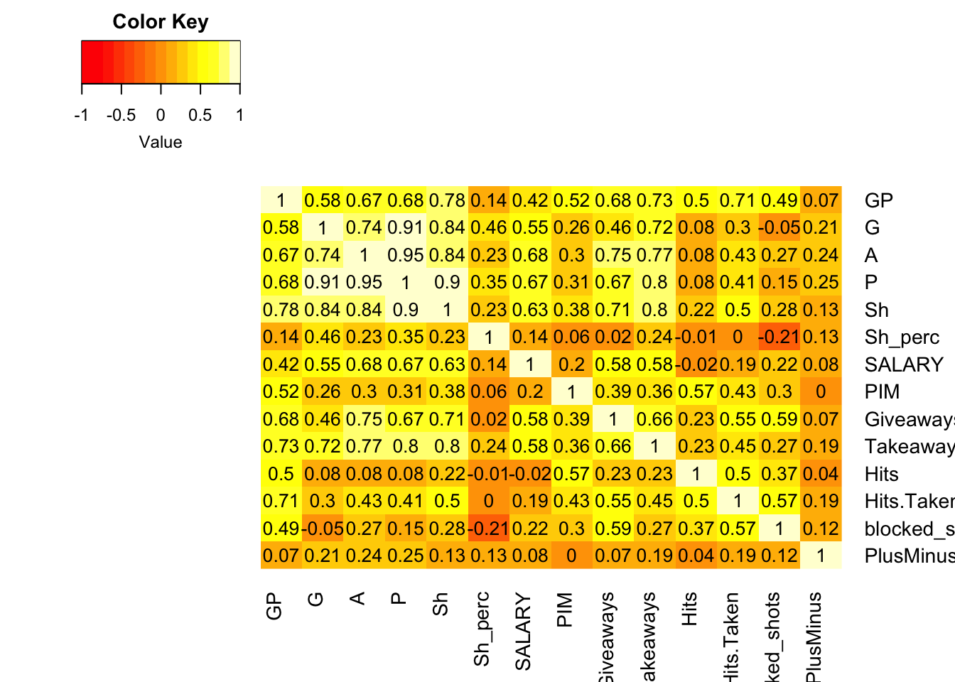

From heatmap we can see correlation value between variables in our dataset. The Goal, Assists number, total shots and number of takeaways and points are strongly correlated between each other (>0.7). The assists number, shots and giveaways number also strongly correlated. While shot percentage negatively impacts blocked shots number, PlusMinus have very small connection with all remaining variables. Here, we can observe multicolinearity since Points is the sum of Goals and Assists, making them dependent variables. Similarly, Shot Percentage is derived by dividing Shots to Goals. Since Shots represent the number of times a player attempts to score, and Points are the sum of goals and assists, these numbers are interconnected. So Shots can cause Goals, and when a player scores a Goal, an Assist should be credited to the player, the sum of these two numbers are represented as Points. Since we can’t use dependent variables as inputs in linear model, let’s keep Points as it holds more value than total shots, as a player may take many shots without successfully scoring a goal. Also it is more correlated to output variable.

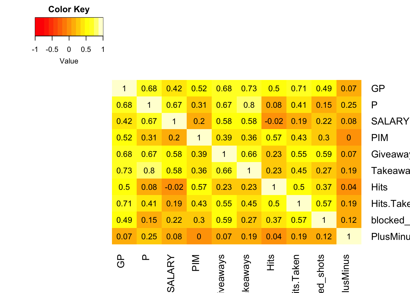
In new heatmap, we can see that Takeaways and Points are highly correlated (=0.8). Maybe these numbers are not dependent, but when player took a puck from an opposite it can lead to goal. Let’s remove Takeaways from our model. The player with high giveaways have a tendency to lose a puck more often, which can decrease team’s performance. Which also can affect Points earned. Also let’s remove Hits.Taken since its highly correlated with Games Played (=0.71). More games played more possibility to make a contact with the player who has the puck. And let’s build model with remaining variables, and use backward elimination.

nhl_train_numbers <- nhl_train_numbers %>% select(-Takeaways, -Giveaways, -Hits.Taken)
nhl_train_numbers %>% cor()

                      GP          P      SALARY         PIM        Hits
GP            1.00000000 0.67582735  0.42421317 0.520448294  0.49558958
P             0.67582735 1.00000000  0.66990334 0.305617550  0.08245484
SALARY        0.42421317 0.66990334  1.00000000 0.198372387 -0.02394758
PIM           0.52044829 0.30561755  0.19837239 1.000000000  0.56542977
Hits          0.49558958 0.08245484 -0.02394758 0.565429770  1.00000000
blocked_shots 0.48789199 0.14605555  0.22171296 0.304039783  0.36510186
PlusMinus     0.07172414 0.24643918  0.07974078 0.003629743  0.03591750
              blocked_shots   PlusMinus
GP                0.4878920 0.071724142
P                 0.1460555 0.246439184
SALARY            0.2217130 0.079740779
PIM               0.3040398 0.003629743
Hits              0.3651019 0.035917499
blocked_shots     1.0000000 0.122277735
PlusMinus         0.1222777 1.000000000

When categorical variables used as predictors, we convert them into dummy variables. A variable with n categories will have n-1 dummy variables, and remaining one value will be as reference level. This helps in analyzing the impact of categorical predictors on the dependent variable.

nhl_train.df <- nhl_train.df %>% select(-G, -A, -Sh, -Sh_perc, -Takeaways, -Giveaways, -Hits.Taken)
nhl_train.df <- nhl_train.df %>% select(-name)

model1 <- step(lm(SALARY~., data = nhl_train.df), direction = "backward")

Start:  AIC=9856.2
SALARY ~ Team + Position + HANDED + GP + P + PIM + Hits + blocked_shots + 
    PlusMinus

                Df       Sum of Sq        RSS    AIC
- Team          60 263015531187124 1.4790e+15 9802.0
- Position       2     39614240556 1.2161e+15 9852.2
- HANDED         1   3453363733890 1.2195e+15 9855.1
- PIM            1   6847508251807 1.2229e+15 9856.1
<none>                             1.2160e+15 9856.2
- Hits           1  16635747374161 1.2327e+15 9858.8
- GP             1  18064821999018 1.2341e+15 9859.2
- PlusMinus      1  38987510345295 1.2550e+15 9864.8
- blocked_shots  1  41997523523384 1.2580e+15 9865.6
- P              1 546410473355975 1.7624e+15 9978.9

Step:  AIC=9801.99
SALARY ~ Position + HANDED + GP + P + PIM + Hits + blocked_shots + 
    PlusMinus

                Df       Sum of Sq        RSS    AIC
- Position       2   2985822004712 1.4820e+15 9798.7
- PIM            1   2443977770222 1.4815e+15 9800.5
- HANDED         1   4399244297709 1.4834e+15 9801.0
<none>                             1.4790e+15 9802.0
- Hits           1  14816636482001 1.4939e+15 9803.3
- GP             1  22027438385796 1.5011e+15 9805.0
- blocked_shots  1  40378661481616 1.5194e+15 9809.0
- PlusMinus      1  42203193555354 1.5212e+15 9809.4
- P              1 689163748993858 2.1682e+15 9928.5

Step:  AIC=9798.67
SALARY ~ HANDED + GP + P + PIM + Hits + blocked_shots + PlusMinus

                Df       Sum of Sq        RSS    AIC
- PIM            1   2493780976016 1.4845e+15 9797.2
- HANDED         1   4714736033909 1.4867e+15 9797.7
<none>                             1.4820e+15 9798.7
- Hits           1  16381671703132 1.4984e+15 9800.4
- GP             1  26188587267788 1.5082e+15 9802.6
- PlusMinus      1  41950294751938 1.5240e+15 9806.0
- blocked_shots  1 110654200590976 1.5927e+15 9820.9
- P              1 699222750683931 2.1812e+15 9926.5

Step:  AIC=9797.23
SALARY ~ HANDED + GP + P + Hits + blocked_shots + PlusMinus

                Df       Sum of Sq        RSS    AIC
- HANDED         1   5021715383231 1.4895e+15 9796.4
<none>                             1.4845e+15 9797.2
- Hits           1  13910288355677 1.4984e+15 9798.4
- GP             1  24706476867436 1.5092e+15 9800.8
- PlusMinus      1  44055357733151 1.5286e+15 9805.1
- blocked_shots  1 112186182042815 1.5967e+15 9819.7
- P              1 723087011778966 2.2076e+15 9928.6

Step:  AIC=9796.37
SALARY ~ GP + P + Hits + blocked_shots + PlusMinus

                Df       Sum of Sq        RSS    AIC
<none>                             1.4895e+15 9796.4
- Hits           1  13058980965199 1.5026e+15 9797.3
- GP             1  25658762191542 1.5152e+15 9800.1
- PlusMinus      1  43964438030890 1.5335e+15 9804.1
- blocked_shots  1 115091536261284 1.6046e+15 9819.4
- P              1 725150613332920 2.2147e+15 9927.6

Below is the summary of our model. I didn’t include name of the player as an input. From the model we can see that Games Played, Hits, PlusMinus have negative impact on salary. Maybe because of the demand to new players, we got negative coef to GP.

summary(model1)

Call:
lm(formula = SALARY ~ GP + P + Hits + blocked_shots + PlusMinus, 
    data = nhl_train.df)

Residuals:
     Min       1Q   Median       3Q      Max 
-5191324 -1186912  -546795  1046568  8061071 

Coefficients:
              Estimate Std. Error t value    Pr(>|t|)    
(Intercept)    1587099     305342   5.198 0.000000354 ***
GP              -24975      10475  -2.384     0.01768 *  
P               118004       9310  12.675     < 2e-16 ***
Hits             -5146       3026  -1.701     0.08990 .  
blocked_shots    21018       4162   5.050 0.000000734 ***
PlusMinus       -36873      11815  -3.121     0.00196 ** 
---
Signif. codes:  0 '***' 0.001 '**' 0.01 '*' 0.05 '.' 0.1 ' ' 1

Residual standard error: 2125000 on 330 degrees of freedom
Multiple R-squared:  0.5012,    Adjusted R-squared:  0.4936 
F-statistic: 66.31 on 5 and 330 DF,  p-value: < 2.2e-16

mean_salary <- mean(nhl_train.df$SALARY)

sst <- sum((nhl_train.df$SALARY - mean_salary)^2)
sst

[1] 2986122868827386

ssr <- sum((model1$fitted.values-mean_salary)^2)
ssr

[1] 1496580443217731

ssr/sst

[1] 0.5011785

The final value is exactly same as r-squared value of the model.

visualize.t(stat=c(-2.384, 2.384), df=330, section="bounded")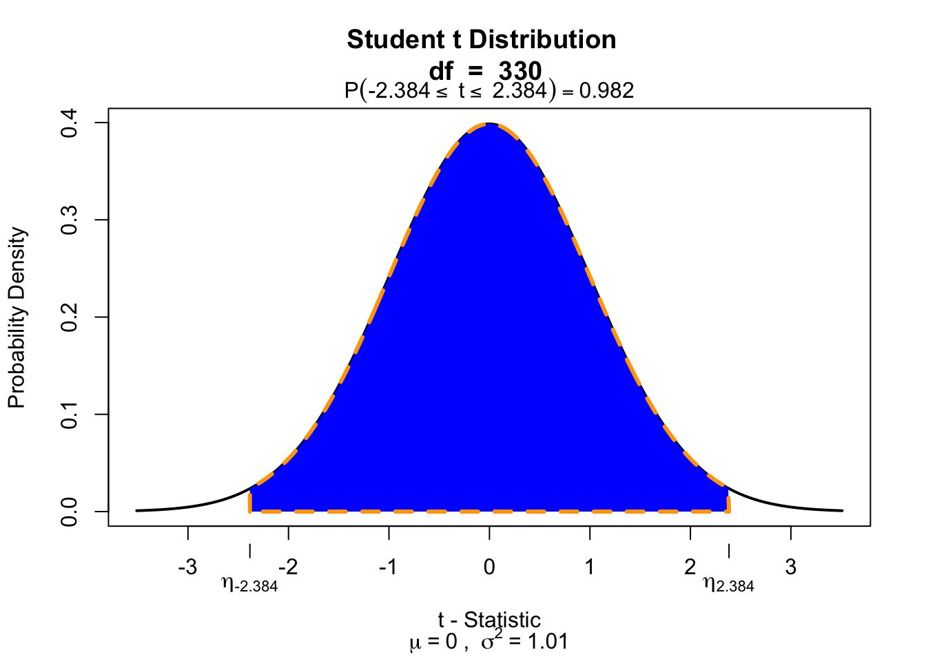

t-value for GP is -2.384. After plotting distribution for that t-value, we can see that 98.2% of the curve is shaded. A bigger t-value occupy more space, and p-value goes lower. The remaining 1.8% (p-value) is the probability of obtaining a t-statistic beyond [-2.384, 2.384].

summary(model1)

Call:
lm(formula = SALARY ~ GP + P + Hits + blocked_shots + PlusMinus, 
    data = nhl_train.df)

Residuals:
     Min       1Q   Median       3Q      Max 
-5191324 -1186912  -546795  1046568  8061071 

Coefficients:
              Estimate Std. Error t value    Pr(>|t|)    
(Intercept)    1587099     305342   5.198 0.000000354 ***
GP              -24975      10475  -2.384     0.01768 *  
P               118004       9310  12.675     < 2e-16 ***
Hits             -5146       3026  -1.701     0.08990 .  
blocked_shots    21018       4162   5.050 0.000000734 ***
PlusMinus       -36873      11815  -3.121     0.00196 ** 
---
Signif. codes:  0 '***' 0.001 '**' 0.01 '*' 0.05 '.' 0.1 ' ' 1

Residual standard error: 2125000 on 330 degrees of freedom
Multiple R-squared:  0.5012,    Adjusted R-squared:  0.4936 
F-statistic: 66.31 on 5 and 330 DF,  p-value: < 2.2e-16

F-statistic: 66.31 F-statistic tests overall significance of the model. The better the fit, the higher the F-score will be.

# F-statistic calculation
k <- 5
n <- 336
sse <- sum(model1$residuals^2)

numerator <- ssr/k
denominator <- sse / (n-k-1)
numerator / denominator

[1] 66.31185

predict(model1, newdata = data.frame(GP=82, P=60, Hits=150, blocked_shots=100, PlusMinus=20))

      1 
7211812 

So, by using the predict() function with random data the predicted salary is $7,211,812. It was found by using Regression Equation: 1587099-24975GP+118004P-5146Hits+21018blocked_shots-36873*PlusMinus

train1 <- predict(model1, nhl_train.df)
valid1 <- predict(model1, nhl_valid.df)

# Training Set
accuracy(train1, nhl_train.df$SALARY)

                        ME    RMSE     MAE       MPE     MAPE
Test set 0.000000004849253 2105508 1592227 -46.79522 72.45567

# Validation Set
accuracy(valid1, nhl_valid.df$SALARY)

              ME    RMSE     MAE       MPE     MAPE
Test set 39476.6 1975654 1532076 -38.84478 64.69072

We got overall measures of predictive accuracy, now for MLR model. RMSE value for validation set (1975654) is also smaller than training set (2105508). Same with MAE, for training set is 1592227, and for validation set is 1532076. Small difference between these numbers can suggest that our model is not overfitting.

2105508/sd(nhl_train.df$SALARY)

[1] 0.7052214

1975654/sd(nhl_train.df$SALARY)

[1] 0.6617279

Compared to SLR, we got smaller coefficients by comparing RMSE to standard deviation of training set. So, using multiple inputs to predict salary is more efficient than using only points. Our model explains 50% of the variance in salary, which suggests there are other factors that can impact salary of the player. As I mentioned earlier, the reputation of the player, and the budget of the team can play major role. These variables not included in our model.