library(tidyverse)
library(dplyr)
library(caret)
library(ggplot2)
library(ggdendro)
library(skimr)
pokemon <- read.csv('all_pokemon_data.csv')Clustering Pokémon: A Hierarchical Approach to Character Grouping
Performed hierarchical clustering on a sample of 20 Pokémon using R. Selected five numeric attributes (e.g., HP, Speed, Attack) and scaled them to build a dendrogram and identify character clusters. Explored both equal-weight and custom-weight variable clustering to observe differences in cluster composition. Used cutree() to assign clusters, visualized relationships with dendrograms, scatterplots, and boxplots, and analyzed cluster traits using summary statistics. Tools used include dplyr, ggplot2, and stats.
This work is part of an assignment for the AD699 Data Mining course.
Data Exploration
dim(pokemon)[1] 1184 24Dataset consists of 1184 rows and 24 columns.
set.seed(79)
random_sample <- pokemon[sample(nrow(pokemon), 20), ]

sum(is.na(random_sample))
[1] 0There is no NA values in random chosen sample.
skim(random_sample)| Name | random_sample |
| Number of rows | 20 |
| Number of columns | 24 |
| _______________________ | |
| Column type frequency: | |
| character | 9 |
| numeric | 15 |
| ________________________ | |
| Group variables | None |
Variable type: character
| skim_variable | n_missing | complete_rate | min | max | empty | n_unique | whitespace |
|---|---|---|---|---|---|---|---|
| Name | 0 | 1 | 5 | 14 | 0 | 20 | 0 |
| Primary.Typing | 0 | 1 | 3 | 8 | 0 | 10 | 0 |
| Secondary.Typing | 0 | 1 | 0 | 6 | 9 | 7 | 0 |
| Secondary.Typing.Flag | 0 | 1 | 4 | 5 | 0 | 2 | 0 |
| Generation | 0 | 1 | 12 | 15 | 0 | 8 | 0 |
| Legendary.Status | 0 | 1 | 4 | 5 | 0 | 2 | 0 |
| Form | 0 | 1 | 4 | 6 | 0 | 3 | 0 |
| Alt.Form.Flag | 0 | 1 | 4 | 5 | 0 | 2 | 0 |
| Color.ID | 0 | 1 | 3 | 5 | 0 | 7 | 0 |
Variable type: numeric
| skim_variable | n_missing | complete_rate | mean | sd | p0 | p25 | p50 | p75 | p100 | hist |
|---|---|---|---|---|---|---|---|---|---|---|
| National.Dex.. | 0 | 1 | 564.10 | 331.92 | 40 | 271.25 | 572.0 | 886.25 | 1001 | ▅▅▃▂▇ |
| Evolution.Stage | 0 | 1 | 1.70 | 0.80 | 1 | 1.00 | 1.5 | 2.00 | 3 | ▇▁▅▁▃ |
| Number.of.Evolution | 0 | 1 | 1.95 | 0.89 | 1 | 1.00 | 2.0 | 3.00 | 3 | ▇▁▅▁▇ |
| Catch.Rate | 0 | 1 | 55.00 | 49.28 | 3 | 41.25 | 47.5 | 75.00 | 235 | ▇▇▁▁▁ |
| Height..dm. | 0 | 1 | 13.15 | 6.18 | 3 | 10.00 | 12.0 | 18.25 | 25 | ▃▇▇▅▂ |
| Weight..hg. | 0 | 1 | 1216.95 | 2004.27 | 3 | 74.25 | 470.0 | 1381.00 | 8000 | ▇▂▁▁▁ |
| Height..in. | 0 | 1 | 51.70 | 24.35 | 12 | 39.00 | 47.0 | 72.00 | 98 | ▃▇▇▅▂ |
| Weight..lbs. | 0 | 1 | 268.35 | 441.84 | 1 | 16.50 | 103.5 | 304.25 | 1764 | ▇▂▁▁▁ |
| Base.Stat.Total | 0 | 1 | 476.70 | 84.69 | 198 | 449.25 | 492.5 | 512.50 | 580 | ▁▁▂▇▆ |
| Health | 0 | 1 | 82.05 | 25.90 | 28 | 68.75 | 82.5 | 100.00 | 140 | ▂▇▇▇▁ |
| Attack | 0 | 1 | 92.50 | 30.02 | 25 | 70.00 | 95.0 | 107.50 | 145 | ▁▇▅▇▅ |
| Defense | 0 | 1 | 79.50 | 30.49 | 25 | 60.00 | 72.5 | 100.00 | 135 | ▅▇▇▅▆ |
| Special.Attack | 0 | 1 | 71.60 | 22.26 | 20 | 58.75 | 72.5 | 86.25 | 112 | ▁▅▇▅▅ |
| Special.Defense | 0 | 1 | 78.05 | 32.10 | 20 | 63.75 | 72.5 | 90.00 | 154 | ▃▇▇▂▂ |
| Speed | 0 | 1 | 73.00 | 25.52 | 30 | 52.50 | 72.5 | 91.25 | 120 | ▇▂▇▇▂ |
Categorical: National.Dex, Evolution.Stage
Numerical: Number.of.Evolution, Catch Rate, Height..dm., Weight..hg., Height..in., Weight..lbs., Base.Stat.Total, Health, Attack, Defense, Special Attack, Special Defense, Speed
rand_sp_numeric <- random_sample %>%
  select (Name, Catch.Rate, Special.Defense, Special.Attack, Speed, Health)
rownames(rand_sp_numeric) <- rand_sp_numeric$Name

rand_sp_numeric
rand_sp_numeric <- rand_sp_numeric %>% select(-Name)Performance indicators can be good options for clustering. Since Base Stat Total already covers other stats, keeping it can cause multicolinerity between variables. Therefore, I excluded Base Stat Total and instead selected a focused set of variables: Speed, Catch Rate, Health, Special Attack, Special Defense. I want to cluster pokemons based on magic-based powerhouses, because of that I chose Special variables. Speed, health, and catch rate help show how fast, tough, or easy to catch a Pokémon is—things that also reflect their overall performance.
| Name | rand_sp_numeric |
| Number of rows | 20 |
| Number of columns | 5 |
| _______________________ | |
| Column type frequency: | |
| numeric | 5 |
| ________________________ | |
| Group variables | None |
Variable type: numeric
| skim_variable | n_missing | complete_rate | mean | sd | p0 | p25 | p50 | p75 | p100 | hist |
|---|---|---|---|---|---|---|---|---|---|---|
| Catch.Rate | 0 | 1 | 55.00 | 49.28 | 3 | 41.25 | 47.5 | 75.00 | 235 | ▇▇▁▁▁ |
| Special.Defense | 0 | 1 | 78.05 | 32.10 | 20 | 63.75 | 72.5 | 90.00 | 154 | ▃▇▇▂▂ |
| Special.Attack | 0 | 1 | 71.60 | 22.26 | 20 | 58.75 | 72.5 | 86.25 | 112 | ▁▅▇▅▅ |
| Speed | 0 | 1 | 73.00 | 25.52 | 30 | 52.50 | 72.5 | 91.25 | 120 | ▇▂▇▇▂ |
| Health | 0 | 1 | 82.05 | 25.90 | 28 | 68.75 | 82.5 | 100.00 | 140 | ▂▇▇▇▁ |
head(rand_sp_numeric)The data needs to be normalized because each column has a different range of values. This makes sure that all variables have equal weight in clustering. Otherwise, the column with higher magnitude - Catch Rate will have higher influence.
norm <- preProcess(rand_sp_numeric, method = c("center", "scale"))
random_sample_norm <- predict(norm, rand_sp_numeric)
random_sample_norm
Hierarchical Clustering
d.norm <- dist(random_sample_norm, method="euclidean")
# d.norm

hc <- hclust(d.norm, method="average")
ggdendrogram(hc) 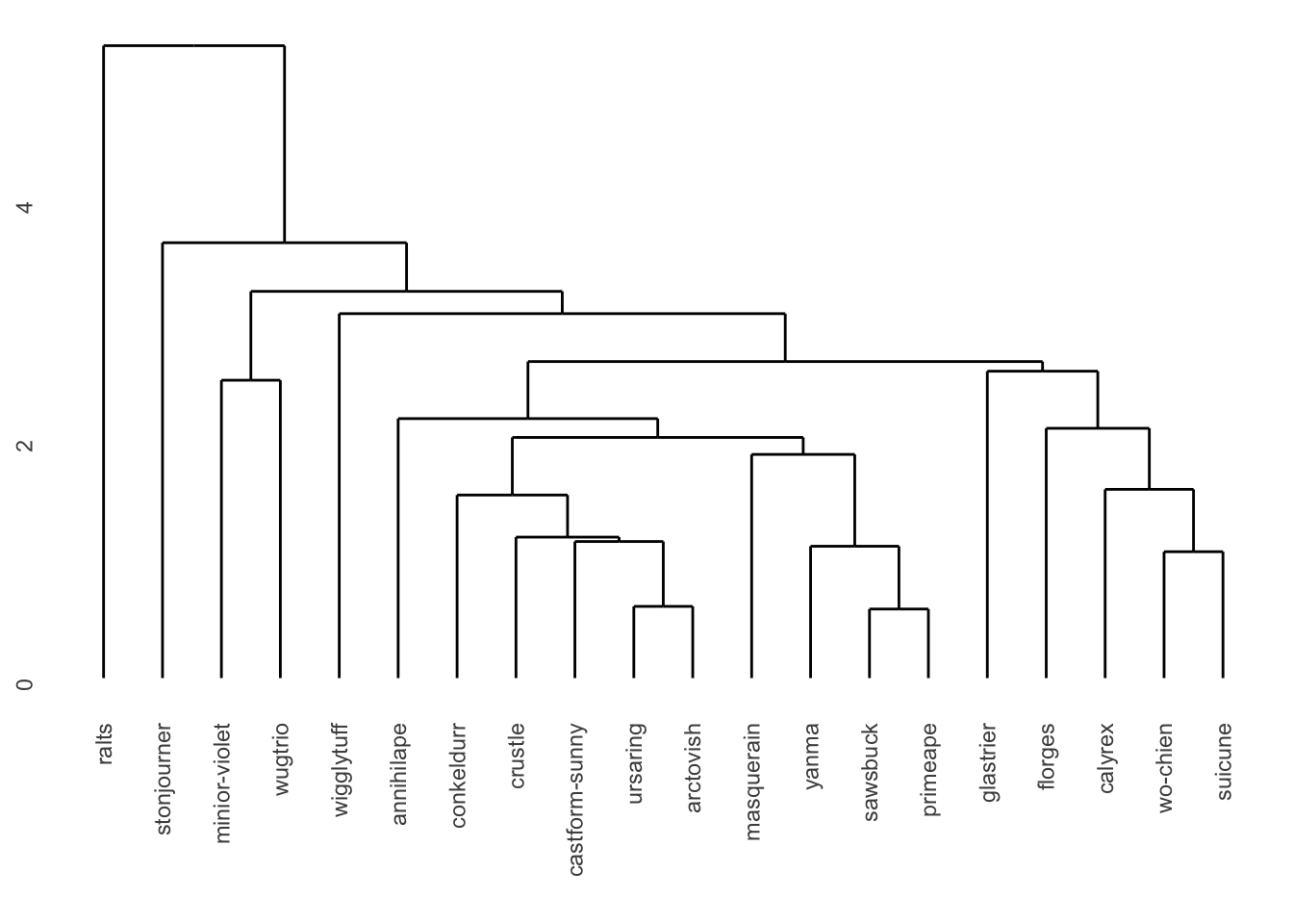
ggdendrogram(hc) +
  geom_hline(yintercept = 3, color = "red", linetype = "dashed")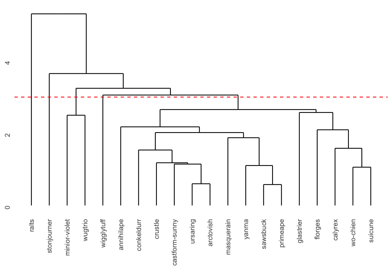
The number of clusters can vary depending on how we interpret the data. If we look for very distinct groups, we can see that the leftmost cluster is clearly separate from the others. Let’s draw a line with cut point=3, and group characters based on that. As a result we get 5 groups: {ralts}, {stonjourner}, {minior-violet and wugtrio}, {wigglytuff}, {others}.
clusters <- cutree(hc, k = 5)
clusters
sawsbuck wo-chien calyrex suicune minior-violet
1 1 1 1 2
conkeldurr annihilape glastrier ursaring yanma
1 1 1 1 1
masquerain ralts castform-sunny stonjourner wugtrio
1 3 1 4 2
crustle florges wigglytuff primeape arctovish
1 1 5 1 1 rand_sp_numeric$cluster <- clusters
cluster_mean <- rand_sp_numeric %>% group_by(cluster) %>%
summarise_all(mean)
cluster_mean# A tibble: 5 × 6
cluster Catch.Rate Special.Defense Special.Attack Speed Health
<int> <dbl> <dbl> <dbl> <dbl> <dbl>
1 1 45 88.4 75.5 71 85.2
2 2 40 65 75 120 47.5
3 3 235 35 45 40 28
4 4 60 20 20 70 100
5 5 50 50 85 45 140 After calculating mean values of each cluster, we see that:
Cluster 1: high special defense; moderate speed, special attack and health; low catch rate. This cluster seems to group defensive Pokemon that are less focused on catching.
Cluster 2: highest speed, lowest catch rate, remaining variables are moderate. This cluster groups fastest Pokemon that are harder to catch, possibly indicating Pokemon with high mobility.
Cluster 3: highest catch rate, while remaining values are low. Seems like this cluster have only one Pokemon, since catch rate is extremely high, which indicates Pokemon that’s easy to catch but weak in battle.
Cluster 4: lowest special defense and attack, health parameter is relatively high and others are moderate. This cluster group Pokemon with high survivability but with low offensive capabilities.
Cluster 5: highest special attack and health values, and others moderate. This cluster groups powerful special attackers with strong survival level.
Data Visualization
rand_sp_numeric$cluster <- factor(rand_sp_numeric$cluster)

ggplot(rand_sp_numeric, aes(x=Speed, y=Catch.Rate, color=cluster)) +
  geom_point()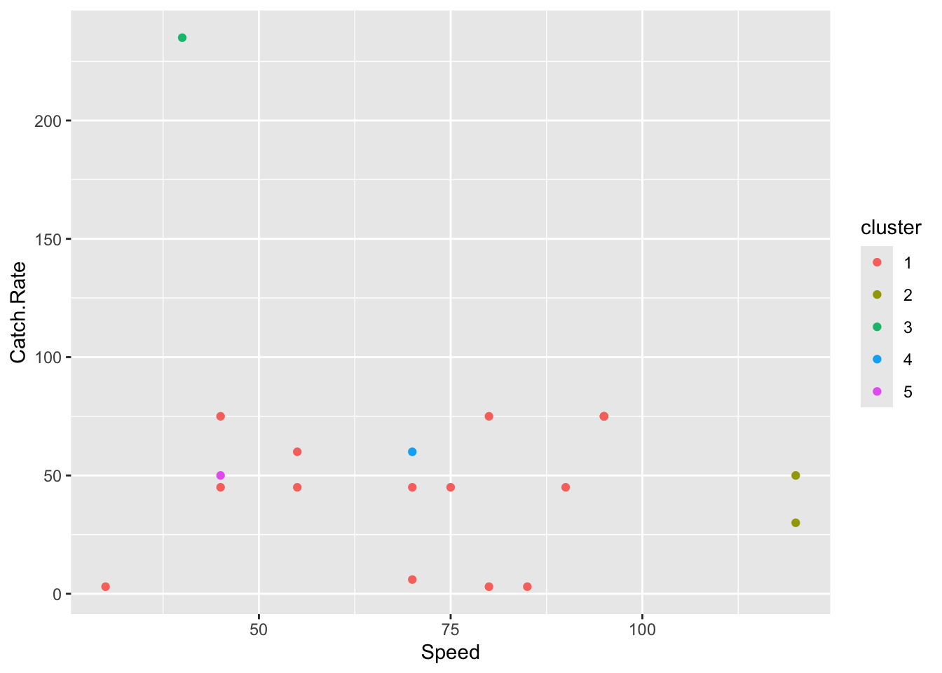
The scatter plot above shows relationship between Speed and Catch Rate across clusters. We can see one Pokemon in Cluster 3 with the highest Catch rate. Although there are two members in CLuster 2 with the highest Speed values.
ggplot(rand_sp_numeric, aes(x=Special.Attack, y=Health, color=cluster)) +
  geom_point()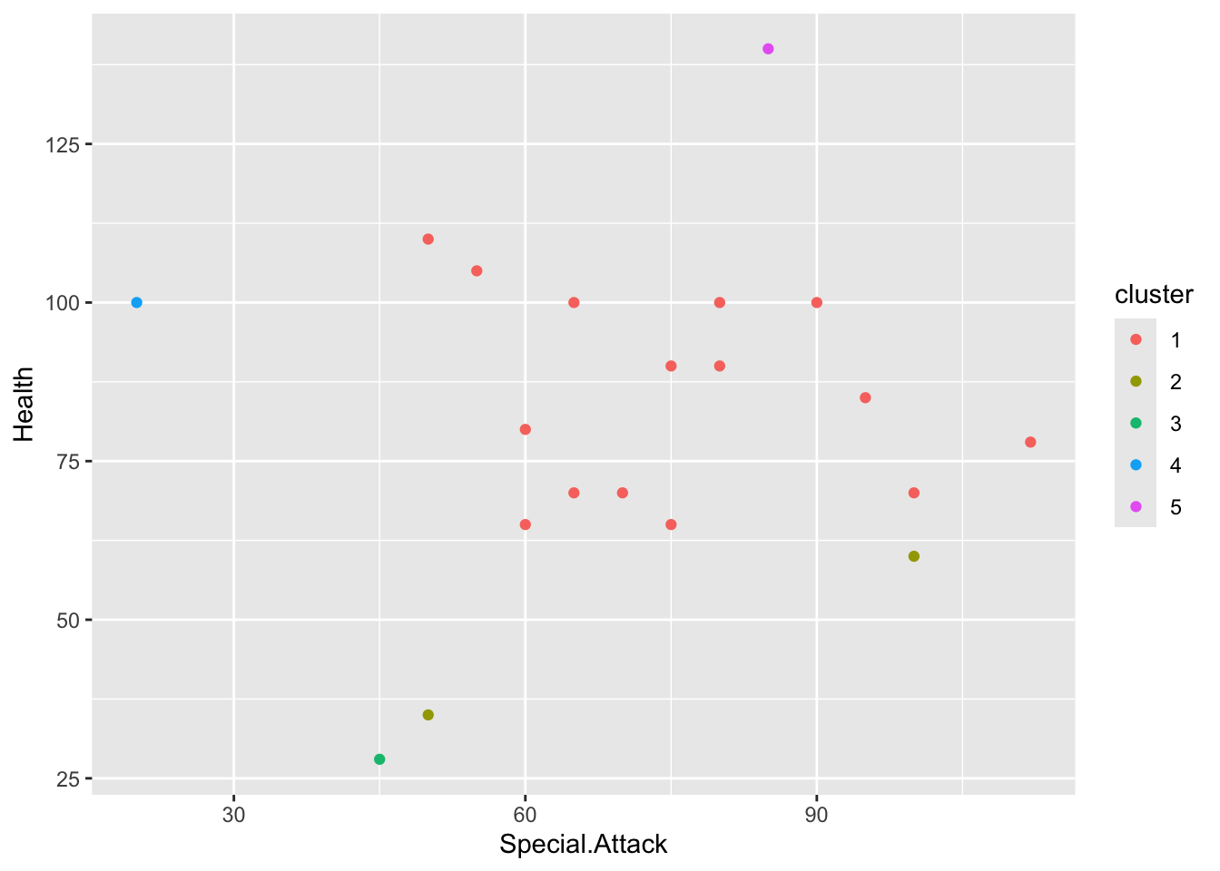
The scatter plot shows the relationship between Health and Special Attack across clusters. We can see that Cluster 1 members have average health and higher special attack, Cluster 4 have one member with lowest special attack and moderate health value. CLuster 5 groups Pokemon with high health and special attack, and Cluster 3 contains Pokemon with lowest health and moderate attack, likely focusing more on offense. Although, Cluster 2 consists of two Pokemon: one with lowest health and moderate attack, another with high attack and moderate health.
ggplot(rand_sp_numeric, aes(x=cluster, y=Speed)) +
  geom_boxplot()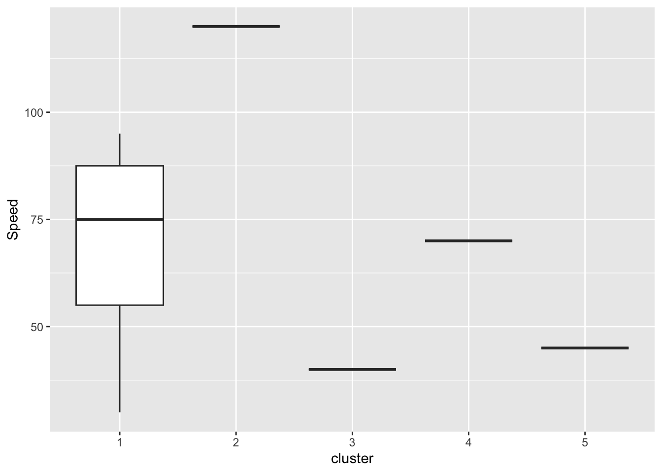
The boxplot above shows distribution of Speed values across clusters. Cluster 1 has a large number of Pokemon, with a broader range of Speed values, while other clusters contains only 1 or 2 Pokemon. When comparing the median Speed values, Cluster 2 has the highest median Speed, indicating that these Pokemon are the fastest. Clusters 3 and 4 have lower median Speed values, meaning that these are slowest ones.
rand_sp_numeric[5,] Catch.Rate Special.Defense Special.Attack Speed Health cluster
minior-violet 30 60 100 120 60 2rand_sp_numeric %>% filter(cluster==2) Catch.Rate Special.Defense Special.Attack Speed Health cluster
minior-violet 30 60 100 120 60 2
wugtrio 50 70 50 120 35 2The Pokemon Minior-violet falls into Cluster 2, group of fastest Pokemon. This cluster contains two Pokemon, both having the similar highest Speed value, making it the key feature in Cluster 2. They also have relatively close special defense values. Although there are large differences in Special Attack and Health, these seem to have less impact compared to their shared high Speed.
Custom Weighting
Equal weighting can be problematic if some parameters are more important than others. If we want the clustering to depend more on certain variables and less on others, giving all features the same weight might not reflect what we’re really trying to group. For example, in this case, I’m more interested in clustering based on special or magical attributes, so those variables should carry more influence.
random_sample.weighted <- random_sample_norm

random_sample.weighted$Special.Attack <- random_sample.weighted$Special.Attack*30
random_sample.weighted$Special.Defense <- random_sample.weighted$Special.Defense*25
random_sample.weighted$Speed <- random_sample.weighted$Speed*20
random_sample.weighted$Health <- random_sample.weighted$Health*10
random_sample.weighted$Catch.Rate <- random_sample.weighted$Catch.Rate*5
Since I want to cluster based on special, magic-based parameters, I assigned weights to the variables accordingly: Special attack is the most important, so it gets a weight of 30. Special defense supports magical resistance, and gets a weight of 25. Speed is useful for overall performance, so I gave it a weight of 20. Health is still important, just less critical here, with a weight of 10. Catch rate has the least impact on magical strength, so it gets a weight of 5.
d.norm2 <- dist(random_sample.weighted, method="euclidean")

hc2 <- hclust(d.norm2, method="average")
ggdendrogram(hc2)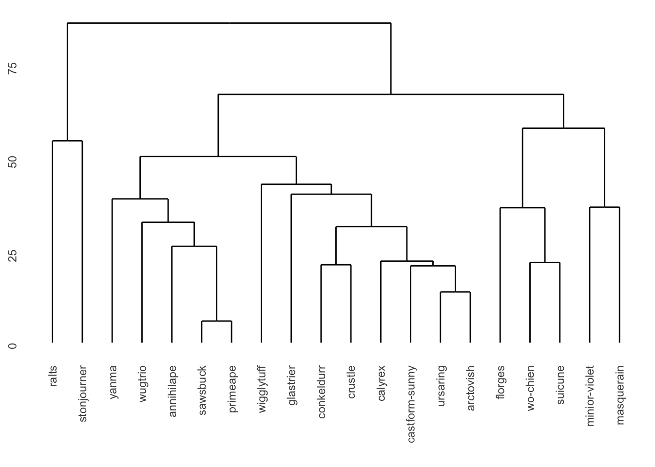
In new dendrogram, the y-axis now ranges from 0 to 75, compared to the previous range of 0 to 4. This shows a wider range of dissimilarity within clusters. Also, there are no singletons in this version — all items are connected to small groups. The way the items cluster together, and the distances at which these groupings happen, are also noticeably different compared to the unweighted version. For instance, before applying weight Pokemon Ralts didn’t belong to any clear group — it was directly connected to all the remaining ones. After applying the weights, Ralts is now grouped with Stonjourner, and together they are then connected to the rest.
clusters2 <- cutree(hc2, k = 4)
clusters2
sawsbuck wo-chien calyrex suicune minior-violet
1 2 1 2 3
conkeldurr annihilape glastrier ursaring yanma
1 1 1 1 1
masquerain ralts castform-sunny stonjourner wugtrio
3 4 1 4 1
crustle florges wigglytuff primeape arctovish
1 2 1 1 1 rand_sp_numeric$cluster <- clusters2
rand_sp_numeric %>% group_by(cluster) %>%
summarise_all(mean)# A tibble: 4 × 6
cluster Catch.Rate Special.Defense Special.Attack Speed Health
<int> <dbl> <dbl> <dbl> <dbl> <dbl>
1 1 49.7 73.8 66.9 70.8 86.2
2 2 18 135. 99 76.7 87.7
3 3 52.5 71 100 100 65
4 4 148. 27.5 32.5 55 64 After grouping Pokemon into 4 groups, some patterns emerge:
Cluster 1: high Health, with other parameters moderate. This group includes Pokemon that are built to last longer in battle, but with less focus on offensive power.
Cluster 2: highest special defense, attack, and health, with the lowest catch rate. These are powerful, magic-based Pokemon that are hard to catch — fitting for their strong battle stats.
Cluster 3: highest special attack and speed, but low health value. These are fast, offensive Pokemon — strong in attack but fragile in battle.
Cluster 4: highest catch rate, with other values low. These are easiest to catch, and tend to be less competitive in battle.
rand_sp_numeric[5,] Catch.Rate Special.Defense Special.Attack Speed Health cluster
minior-violet 30 60 100 120 60 3rand_sp_numeric %>% filter(cluster==3) Catch.Rate Special.Defense Special.Attack Speed Health cluster
minior-violet 30 60 100 120 60 3
masquerain 75 82 100 80 70 3After weighting, Minior-violet was moved to Cluster 3, which also contains two Pokemon. The other member of this cluster has the same Special Attack value, similar Health, and both share a high Speed value. Before weighting, Minior-violet was placed in Cluster 2, where its highest Speed value was the key feature driving the grouping. After weighting, special attack and defense were given more importance. This made Minior-violet more similar to Masquerain, which shares those characteristics of high Special Attack and Speed, even though both Pokémon have relatively low Health.