library(tidyverse)
library(dplyr)
library(skimr)
library(caret)
library(FNN)
library(ggplot2)

spotify_2023 <- read.csv('spotify-2023.csv')K-Nearest Neighbors: You Like This Song…But Will George Like It?
In this project, I’ll use k-NN clustering analysis to find out whether George—a fictional character—would vibe with my song or not.
This work is part of an assignment for the AD699 Data Mining course.
str(spotify_2023)'data.frame': 953 obs. of 24 variables:
$ track_name : chr "Seven (feat. Latto) (Explicit Ver.)" "LALA" "vampire" "Cruel Summer" ...
$ artist.s._name : chr "Latto, Jung Kook" "Myke Towers" "Olivia Rodrigo" "Taylor Swift" ...
$ artist_count : int 2 1 1 1 1 2 2 1 1 2 ...
$ released_year : int 2023 2023 2023 2019 2023 2023 2023 2023 2023 2023 ...
$ released_month : int 7 3 6 8 5 6 3 7 5 3 ...
$ released_day : int 14 23 30 23 18 1 16 7 15 17 ...
$ in_spotify_playlists: int 553 1474 1397 7858 3133 2186 3090 714 1096 2953 ...
$ in_spotify_charts : int 147 48 113 100 50 91 50 43 83 44 ...
$ streams : chr "141381703" "133716286" "140003974" "800840817" ...
$ in_apple_playlists : int 43 48 94 116 84 67 34 25 60 49 ...
$ in_apple_charts : int 263 126 207 207 133 213 222 89 210 110 ...
$ in_deezer_playlists : chr "45" "58" "91" "125" ...
$ in_deezer_charts : int 10 14 14 12 15 17 13 13 11 13 ...
$ in_shazam_charts : chr "826" "382" "949" "548" ...
$ bpm : int 125 92 138 170 144 141 148 100 130 170 ...
$ key : chr "B" "C#" "F" "A" ...
$ mode : chr "Major" "Major" "Major" "Major" ...
$ danceability_. : int 80 71 51 55 65 92 67 67 85 81 ...
$ valence_. : int 89 61 32 58 23 66 83 26 22 56 ...
$ energy_. : int 83 74 53 72 80 58 76 71 62 48 ...
$ acousticness_. : int 31 7 17 11 14 19 48 37 12 21 ...
$ instrumentalness_. : int 0 0 0 0 63 0 0 0 0 0 ...
$ liveness_. : int 8 10 31 11 11 8 8 11 28 8 ...
$ speechiness_. : int 4 4 6 15 6 24 3 4 9 33 ...My song is Money Trees - Kendrick Lamar, Jay Rock. I’m a big fan of Kendrick’s music, and especially songs from this album is one of the favorites of mine.
Here is the values of this song from dataset:
danceability: 74
energy: 53
speechiness: 10
acousticness: 7
liveness: 21
valence: 37
BPM: 144
my_song <- spotify_2023 %>% filter(track_name == 'Money Trees')
my_song
spotify <- read.csv('spotify.csv')
str(spotify)'data.frame': 2017 obs. of 17 variables:
$ X : int 0 1 2 3 4 5 6 7 8 9 ...
$ acousticness : num 0.0102 0.199 0.0344 0.604 0.18 0.00479 0.0145 0.0202 0.0481 0.00208 ...
$ danceability : num 0.833 0.743 0.838 0.494 0.678 0.804 0.739 0.266 0.603 0.836 ...
$ duration_ms : int 204600 326933 185707 199413 392893 251333 241400 349667 202853 226840 ...
$ energy : num 0.434 0.359 0.412 0.338 0.561 0.56 0.472 0.348 0.944 0.603 ...
$ instrumentalness: num 2.19e-02 6.11e-03 2.34e-04 5.10e-01 5.12e-01 0.00 7.27e-06 6.64e-01 0.00 0.00 ...
$ key : int 2 1 2 5 5 8 1 10 11 7 ...
$ liveness : num 0.165 0.137 0.159 0.0922 0.439 0.164 0.207 0.16 0.342 0.571 ...
$ loudness : num -8.79 -10.4 -7.15 -15.24 -11.65 ...
$ mode : int 1 1 1 1 0 1 1 0 0 1 ...
$ speechiness : num 0.431 0.0794 0.289 0.0261 0.0694 0.185 0.156 0.0371 0.347 0.237 ...
$ tempo : num 150.1 160.1 75 86.5 174 ...
$ time_signature : num 4 4 4 4 4 4 4 4 4 4 ...
$ valence : num 0.286 0.588 0.173 0.23 0.904 0.264 0.308 0.393 0.398 0.386 ...
$ target : int 1 1 1 1 1 1 1 1 1 1 ...
$ song_title : chr "Mask Off" "Redbone" "Xanny Family" "Master Of None" ...
$ artist : chr "Future" "Childish Gambino" "Future" "Beach House" ...spotify$target <- factor(spotify$target)
levels(spotify$target)[1] "0" "1"table(spotify$target)
   0    1
 997 1020
Data Exploration
Target variable is of type int, then I converted it to categorical variable (factor).
The target factor variable has 2 categories: 0 or 1. By counting total number of rows for each category, we get that George has 1020 favorite, and 997 disliked songs. Which is interesting, that number of disliked ones pretty close to liked. The music taste of George can be diverse, and Spotify’s recommendation system might be actively adjusting to his preferences. Actually, when you dislike one song in Spotify, the system tries to not suggest you similar songs, and try other different options. To state this opinion constantly we need to explore more about song preferences of George. Furthermore, there are could be temporal patterns in George’s preferences, for instance he prefer certain types of songs at different times of day, month or year.
colSums(is.na(spotify)) X acousticness danceability duration_ms
0 0 0 0
energy instrumentalness key liveness
0 0 0 0
loudness mode speechiness tempo
0 0 0 0
time_signature valence target song_title
0 0 0 0
artist
0 There is no NA values in this dataset.
skim(spotify_2023)| Name | spotify_2023 |
| Number of rows | 953 |
| Number of columns | 24 |
| _______________________ | |
| Column type frequency: | |
| character | 7 |
| numeric | 17 |
| ________________________ | |
| Group variables | None |
Variable type: character
| skim_variable | n_missing | complete_rate | min | max | empty | n_unique | whitespace |
|---|---|---|---|---|---|---|---|
| track_name | 0 | 1 | 2 | 123 | 0 | 943 | 0 |
| artist.s._name | 0 | 1 | 1 | 117 | 0 | 645 | 0 |
| streams | 0 | 1 | 4 | 102 | 0 | 949 | 0 |
| in_deezer_playlists | 0 | 1 | 1 | 6 | 0 | 348 | 0 |
| in_shazam_charts | 0 | 1 | 0 | 5 | 50 | 199 | 0 |
| key | 0 | 1 | 0 | 2 | 95 | 12 | 0 |
| mode | 0 | 1 | 5 | 5 | 0 | 2 | 0 |
Variable type: numeric
| skim_variable | n_missing | complete_rate | mean | sd | p0 | p25 | p50 | p75 | p100 | hist |
|---|---|---|---|---|---|---|---|---|---|---|
| artist_count | 0 | 1 | 1.56 | 0.89 | 1 | 1 | 1 | 2 | 8 | ▇▁▁▁▁ |
| released_year | 0 | 1 | 2018.24 | 11.12 | 1930 | 2020 | 2022 | 2022 | 2023 | ▁▁▁▁▇ |
| released_month | 0 | 1 | 6.03 | 3.57 | 1 | 3 | 6 | 9 | 12 | ▇▆▅▃▆ |
| released_day | 0 | 1 | 13.93 | 9.20 | 1 | 6 | 13 | 22 | 31 | ▇▅▃▆▃ |
| in_spotify_playlists | 0 | 1 | 5200.12 | 7897.61 | 31 | 875 | 2224 | 5542 | 52898 | ▇▁▁▁▁ |
| in_spotify_charts | 0 | 1 | 12.01 | 19.58 | 0 | 0 | 3 | 16 | 147 | ▇▁▁▁▁ |
| in_apple_playlists | 0 | 1 | 67.81 | 86.44 | 0 | 13 | 34 | 88 | 672 | ▇▁▁▁▁ |
| in_apple_charts | 0 | 1 | 51.91 | 50.63 | 0 | 7 | 38 | 87 | 275 | ▇▃▂▁▁ |
| in_deezer_charts | 0 | 1 | 2.67 | 6.04 | 0 | 0 | 0 | 2 | 58 | ▇▁▁▁▁ |
| bpm | 0 | 1 | 122.54 | 28.06 | 65 | 100 | 121 | 140 | 206 | ▃▇▇▃▁ |
| danceability_. | 0 | 1 | 66.97 | 14.63 | 23 | 57 | 69 | 78 | 96 | ▁▃▆▇▃ |
| valence_. | 0 | 1 | 51.43 | 23.48 | 4 | 32 | 51 | 70 | 97 | ▅▇▇▇▅ |
| energy_. | 0 | 1 | 64.28 | 16.55 | 9 | 53 | 66 | 77 | 97 | ▁▂▅▇▃ |
| acousticness_. | 0 | 1 | 27.06 | 26.00 | 0 | 6 | 18 | 43 | 97 | ▇▃▂▁▁ |
| instrumentalness_. | 0 | 1 | 1.58 | 8.41 | 0 | 0 | 0 | 0 | 91 | ▇▁▁▁▁ |
| liveness_. | 0 | 1 | 18.21 | 13.71 | 3 | 10 | 12 | 24 | 97 | ▇▂▁▁▁ |
| speechiness_. | 0 | 1 | 10.13 | 9.91 | 2 | 4 | 6 | 11 | 64 | ▇▁▁▁▁ |
spotify_2023$danceability_. <- spotify_2023$danceability_./100
spotify_2023$energy_. <- spotify_2023$energy_./100
spotify_2023$speechiness_. <- spotify_2023$speechiness_./100
spotify_2023$valence_. <- spotify_2023$valence_./100
spotify_2023$acousticness_. <- spotify_2023$acousticness_./100
spotify_2023$liveness_. <- spotify_2023$liveness_./100

spotify_2023 <- spotify_2023 %>% rename(danceability=danceability_., energy=energy_., speechiness=speechiness_., valence=valence_., acousticness=acousticness_., liveness=liveness_., tempo=bpm)

my_song <- spotify_2023 %>% filter(track_name == 'Money Trees')
I converted the values in spotify_23 to decimal format. Also, applied the same changes to my_song by recreating it.
Data Partition
set.seed(79)
spotify.index <- sample(c(1:nrow(spotify)), nrow(spotify)*0.6)
spotify_train.df <- spotify[spotify.index, ]
spotify_valid.df <- spotify[-spotify.index, ]
liked <- spotify_train.df %>% filter(target==1)
disliked <- spotify_train.df %>% filter(target==0)
t.test(liked$danceability, disliked$danceability)
    Welch Two Sample t-test

data:  liked$danceability and disliked$danceability
t = 5.9297, df = 1198.7, p-value = 3.965e-09
alternative hypothesis: true difference in means is not equal to 0
95 percent confidence interval:
 0.03618685 0.07197390
sample estimates:
mean of x mean of y
0.6451020 0.5910216 t.test(liked$tempo, disliked$tempo)
    Welch Two Sample t-test

data:  liked$tempo and disliked$tempo
t = 0.32976, df = 1188, p-value = 0.7416
alternative hypothesis: true difference in means is not equal to 0
95 percent confidence interval:
 -2.495354  3.503627
sample estimates:
mean of x mean of y
121.3866 120.8825 t.test(liked$energy, disliked$energy)
    Welch Two Sample t-test

data:  liked$energy and disliked$energy
t = 0.90709, df = 1116.6, p-value = 0.3646
alternative hypothesis: true difference in means is not equal to 0
95 percent confidence interval:
 -0.01228227  0.03340286
sample estimates:
mean of x mean of y
0.6986168 0.6880565 t.test(liked$speechiness, disliked$speechiness)
    Welch Two Sample t-test

data:  liked$speechiness and disliked$speechiness
t = 5.9565, df = 1102.5, p-value = 3.461e-09
alternative hypothesis: true difference in means is not equal to 0
95 percent confidence interval:
 0.01988822 0.03942699
sample estimates:
 mean of x  mean of y
0.10598684 0.07632924 t.test(liked$valence, disliked$valence)
    Welch Two Sample t-test

data:  liked$valence and disliked$valence
t = 3.4455, df = 1207.9, p-value = 0.0005895
alternative hypothesis: true difference in means is not equal to 0
95 percent confidence interval:
 0.02065933 0.07529932
sample estimates:
mean of x mean of y
0.5254077 0.4774284 t.test(liked$acousticness, disliked$acousticness)
    Welch Two Sample t-test

data:  liked$acousticness and disliked$acousticness
t = -4.0701, df = 1122.3, p-value = 5.028e-05
alternative hypothesis: true difference in means is not equal to 0
95 percent confidence interval:
 -0.08721203 -0.03047773
sample estimates:
mean of x mean of y
0.1508101 0.2096550 t.test(liked$liveness, disliked$liveness)
    Welch Two Sample t-test

data:  liked$liveness and disliked$liveness
t = 1.5056, df = 1192.1, p-value = 0.1324
alternative hypothesis: true difference in means is not equal to 0
95 percent confidence interval:
 -0.004181182  0.031773731
sample estimates:
mean of x mean of y
0.1991905 0.1853942
Based on the results above, here is the list of variables that show significant difference: Danceability(p_value = 3.965e-09), speechiness(p-value = 3.461e-09), valence(p-value = 0.0005895), acousticness(p-value = 5.028e-05). Very low p-value suggests that, there is significant difference on this values between liked and disliked songs, making them main parameters to identify George’s preferences in music. Other remaining variables have p-value more than typical threshold 0.05: tempo(p-value = 0.7416), energy(p-value = 0.3646), liveness(p-value = 0.1324).
spotify_train.df <- spotify_train.df %>% select(-tempo, -energy, -liveness)k-NN method draws information from similarities between the variables by measuring distance between records. Variables with similar values across different outcome classes cannot provide useful information for distinguishing between groups. Including such variables can lead to overfitting, where the model performs well on training data but fails to generalize to new data. These insignificant variables affect the distance calculation, making it harder to distinguish between groups.
head(spotify_train.df)Normalization
In this step we are normalizing only those columns that will be used in k-NN model building.
spotify_train_norm.df <- spotify_train.df
spotify_valid_norm.df <- spotify_valid.df
spotify_norm.df <- spotify
my_song_norm <- my_song


norm_values <- preProcess(
  spotify_train.df[, c("acousticness", "danceability", "speechiness", "valence")],
  method = c("center", "scale"))

spotify_train_norm.df[, c("acousticness", "danceability", "speechiness", "valence")] <-
  predict(norm_values, spotify_train.df[, c("acousticness", "danceability", "speechiness", "valence")])
# View(spotify_train_norm.df)

spotify_valid_norm.df[, c("acousticness", "danceability", "speechiness", "valence")] <-
  predict(norm_values, spotify_valid.df[, c("acousticness", "danceability", "speechiness", "valence")])
# View(spotify_valid_norm.df)

spotify_norm.df[, c("acousticness", "danceability", "speechiness", "valence")] <-
  predict(norm_values, spotify[, c("acousticness", "danceability", "speechiness", "valence")])
# View(spotify_norm.df)

my_song_norm[, c("acousticness", "danceability", "speechiness", "valence")] <-
predict(norm_values, my_song[, c("acousticness", "danceability", "speechiness", "valence")])print(my_song_norm)Clustering
# knn is all about numeric data, classification using numeric values
nn <- knn( train = spotify_train_norm.df[, c("acousticness", "danceability", "speechiness", "valence")],
           test = my_song_norm[, c("acousticness", "danceability", "speechiness", "valence")],
           cl = spotify_train_norm.df[,c("target")],##what we are classifying: like or dislike
           k=7)
print(nn)
[1] 1
attr(,"nn.index")
[,1] [,2] [,3] [,4] [,5] [,6] [,7]
[1,] 823 966 277 929 653 984 436
attr(,"nn.dist")
[,1] [,2] [,3] [,4] [,5] [,6] [,7]
[1,] 0.0233238 0.3074891 0.3136877 0.3537573 0.4308537 0.471654 0.4811864
Levels: 1nn_indexes <- row.names(spotify_train.df)[attr(nn, "nn.index")]
spotify_train.df[nn_indexes, ] %>% select(song_title, artist, target, acousticness, danceability, speechiness, valence)By running k-NN model as a result get “1”, which indicates that George will like my song. And by listing 7 nearest neighbors, I see that my song is also in this list and George already marked it as favorite. Within this songs, George marked only one song as disliked, which highlights not all similar songs are guaranteed to be liked. This disliked song has high valence value compared to others, but there is no difference in other variables. By running knn classification we get 7 nearest records with low distance value from our selected song. So if we just use numbers these songs look very similar to each other. But they are not. And the diversity of artists suggests George’s musical preferences are varied.
accuracy.df <- data.frame(k = seq(1,14,1), accuracy = rep(0,14))

for(i in 1:14) {
  knn.pred <- knn( train = spotify_train_norm.df[, c("acousticness", "danceability", "speechiness", "valence")],
           test = spotify_valid_norm.df[, c("acousticness", "danceability", "speechiness", "valence")],
           cl = spotify_train_norm.df[,c("target")],
           k=i)

  accuracy.df[i, 2] <- confusionMatrix(knn.pred, spotify_valid_norm.df[ ,c("target")])$overall['Accuracy']
}

accuracy.df[order(-accuracy.df$accuracy), ]
k accuracy
14 14 0.6183395
12 12 0.6096654
13 13 0.6096654
10 10 0.6084263
11 11 0.6034696
5 5 0.6022305
9 9 0.5997522
4 4 0.5972739
6 6 0.5960347
8 8 0.5947955
3 3 0.5885998
7 7 0.5861214
1 1 0.5774473
2 2 0.5662949From the list above we can see accuracy for different k values between 1 and 14. We can see that the difference in accuracy between values is very small. k=14 has highest accuracy value 0.6183395, also k=5 provides very similar number 0.6022305.
ggplot(accuracy.df, aes(x=k, y=accuracy)) +
  geom_point() +
  geom_line() +
  labs(title = "Scatterplot of k values vs Accuracy",
       x = "k values",
       y = "Accuracy") +
  scale_x_continuous(breaks = seq(min(accuracy.df$k), max(accuracy.df$k), by = 3))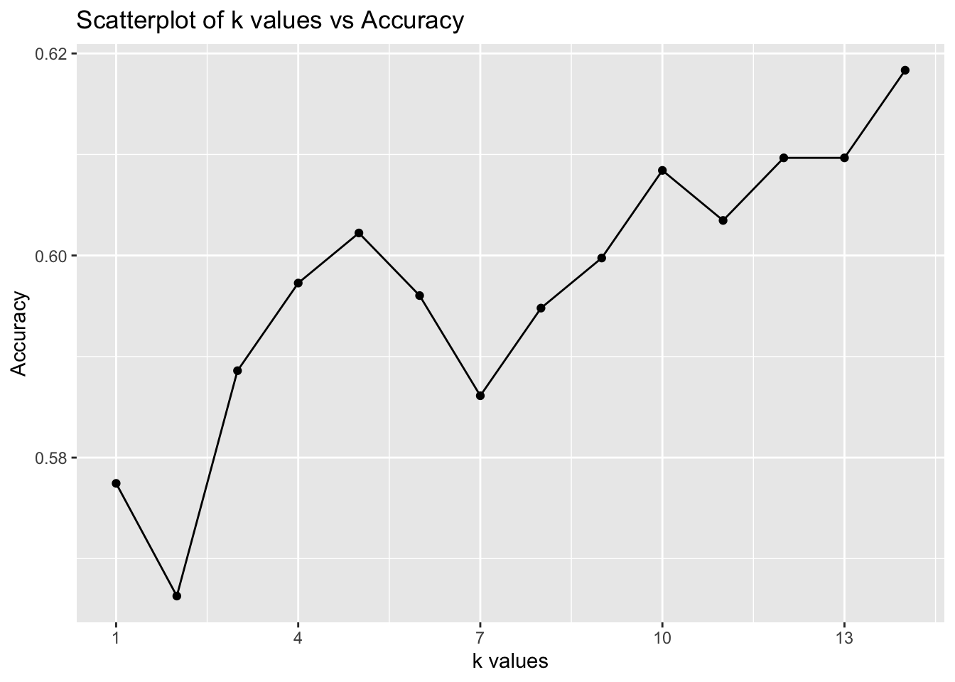
The graph clearly illustrates the differences in accuracy across various k-values. k = 10 has about 61% accuracy, similar to k = 12 and k = 13. Since they give the same result, k = 10 is a better choice to reduce noise. Additionally, the previously used k = 7 had one of the lowest accuracy scores at 59%. While k = 14 had the highest accuracy at 62%, k = 10 appears to be a more balanced choice. Selecting 10 nearest neighbors should provide a more reliable classification of my song.
nn_10 <- knn( train = spotify_train_norm.df[, c("acousticness", "danceability", "speechiness", "valence")],
           test = my_song_norm[, c("acousticness", "danceability", "speechiness", "valence")],
           cl = spotify_train_norm.df[,c("target")],##what we are classifying: like or dislike
           k=10)
print(nn_10)
[1] 1
attr(,"nn.index")
[,1] [,2] [,3] [,4] [,5] [,6] [,7] [,8] [,9] [,10]
[1,] 823 966 277 929 653 984 436 476 136 127
attr(,"nn.dist")
[,1] [,2] [,3] [,4] [,5] [,6] [,7]
[1,] 0.0233238 0.3074891 0.3136877 0.3537573 0.4308537 0.471654 0.4811864
[,8] [,9] [,10]
[1,] 0.501667 0.5050047 0.5092467
Levels: 1nn_indexes_10 <- row.names(spotify_train.df)[attr(nn_10, "nn.index")]
spotify_train.df[nn_indexes_10, ] %>% select(song_title, artist, target, acousticness, danceability, speechiness, valence)I chose k=10 as optimal with moderate accuracy value. The output of model didn’t change, it indicates George will like my song. But for now I got 10 nearest neighbors, and from this new list George disliked 3 songs. All these songs have high value of danceability around 70%, low speechiness and acousticness. All 3 disliked songs as for k=7, have higher value of valence compared to others. Higher valence indicates more positive, cheerful, or euphoric songs. It seems that George might prefer songs with lower valence, which are less positive, more neutral in mood or moodier over cheerful ones. Disliked songs have relatively low acousticness, this suggest that George prefer songs with slightly more acoustic elements. The danceability is quite similar for both groups, which implies this factor is not strong in determining preferences. The disliked songs have relatively low speechiness, and some liked songs have higher speechiness (‘Pacifier’ has 0.1240) indicating George prefer songs with more spoken lyrics or rap.
Limitations of model
I think main limitation here is that we are relying on numerical variables to predict whether someone will like this song or not. There are can be other factors such as good memories or associations with a song which can make them favorite. Also lyrics play main role in connecting with listeners on an emotional level. For instance, I tend to prefer songs with meaningful lyrics, while rap elements often give me an energy boost. Additionally, music preferences can vary based on context—what I listen to at the gym or while walking differs from what I play in the evening when I can’t sleep.