library(tidytext)
library(tidyr)
library(dplyr)
library(ggplot2)
library(reshape2)
library(textdata)
library(wordcloud)
bb <- read.csv("BB_data.csv")Say my name: Unpacking Emotion and Language in Breaking Bad Using R
Applied natural language processing techniques to a single episode of Breaking Bad using R. Conducted frequency analysis to identify top characters by line count, explored most common words and bigrams, and visualized key terms with a wordcloud. Performed sentiment analysis using Bing and AFINN lexicons to assess the emotional tone of the episode. Tools used include dplyr, tidytext, ggplot2, and wordcloud.
This work is part of an assignment for the AD699 Data Mining course.
Text Mining
str(bb)'data.frame': 5641 obs. of 5 variables:
$ actor : chr "Walter" "Skyler" "Walter" "Skyler" ...
$ text : chr "My name is Walter Hartwell White. I live at 308 Negra Arroyo Lane Albuquerque, New Mexico, 87104. To all law en"| __truncated__ "Happy Birthday." "Look at that." "That is veggie bacon. Believe it or not. Zero cholesterol. You won't even taste the difference. What time do yo"| __truncated__ ...
$ season : int 1 1 1 1 1 1 1 1 1 1 ...
$ episode: int 1 1 1 1 1 1 1 1 1 1 ...
$ title : chr "The Pilot" "The Pilot" "The Pilot" "The Pilot" ...my_data <- bb %>% filter(season==1 & episode==5)
head(my_data)top_10 <- my_data %>%
count(actor, sort = TRUE) %>%
slice(1:10)
my_data <- my_data %>% filter(actor %in% top_10$actor) %>%
mutate(actor = factor(actor, levels = top_10$actor))
ggplot(my_data) + geom_bar(aes(y = actor))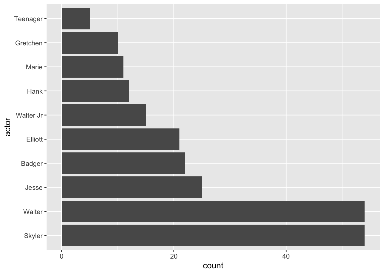
From the barplot above, we can see that Walter and Skyler have similar number of lines in Episode 5 Season 1, suggesting that they are the main characters here. They are followed by Jesse, Badger, and Elliot - most likely supporting characters who have shorter lines but appears alongside with main ones. Other remaining characters each have less than 20 lines, so they probably only showed up briefly or had minor roles in this episode.
my_data_txt <- my_data %>% select(text)

tidy_const <- my_data_txt %>% unnest_tokens(word, text)
tidy_const %>% count(word, sort=TRUE) %>% head(10)
word n
1 you 154
2 i 116
3 to 92
4 the 86
5 it 60
6 a 58
7 what 52
8 and 43
9 this 41
10 that 39After extracting 10 most frequently used words, we mostly ended up with common pronouns like “you”, “I”, “and”, “these”, “that”. These are known as stop words—common terms that appear frequently across most texts. Since they don’t provide any insight into the context of the episode, they are not useful at all.
# stop_words
tidy_const <- my_data_txt %>% unnest_tokens(word, text) %>% anti_join(stop_words)
tidy_const %>% count(word, sort=TRUE) %>% slice(1:10)
word n
1 walt 21
2 elliott 11
3 yeah 11
4 talking 10
5 hey 9
6 skyler 8
7 yo 8
8 gonna 7
9 treatment 7
10 guy 6After removing stopwords, we extracted a different set of words. From the list we can see names of characters, like Walt, Elliiot, Skyler, which are can be main characters like we mentioned previously. Also, it contains less meaningful words like “yeah”, “yo”, “hey”.
tidy_const2 <- my_data_txt %>% unnest_tokens(output = bigram, input=text, token="ngrams", n=2)
tidy_const2 %>% count(bigram, sort=TRUE) %>% slice(1:10)
bigram n
1 you know 19
2 <NA> 16
3 are you 12
4 i mean 12
5 to do 12
6 thank you 11
7 this is 11
8 i don't 10
9 all right 7
10 and i 7Bigrams is combination of two (bi) consecutive words, while unigrams are single words. Bigrams help to get more meaningful insights into context compared to unigrams. For example, the word “pillow” on its own just refers to an object, but the bigram “talking pillow” suggests something very different and more specific. By looking at pairs of words, we can better understand the meaning and flow of the text.
bigrams_sep <- tidy_const2 %>% separate(bigram, c("word1", "word2"), sep = " ")
bigrams_filtered <- bigrams_sep %>% filter(!word1 %in% stop_words$word) %>%
  filter(!word2 %in% stop_words$word) %>%
  filter(!is.na(word1) | !is.na(word2)) %>%
  count(word1, word2, sort = TRUE)
# bigrams_filtered
bigrams_united <- bigrams_filtered %>% unite(col = bigram, word1, word2, sep=" ")
bigrams_united %>% slice(1:10)
bigram n
1 snot trough 3
2 talking pillow 3
3 fat guy 2
4 gray matter 2
5 husband's life 2
6 shit hand 2
7 walter jr 2
8 40 pills 1
9 9th bases 1
10 absolutely miserable 1After extracting bigrams, the initial results included common phrases like “are you” and “this is,” as well as some NA values. These aren’t very meaningful on their own. However, after applying filters we ended up with a more useful and insightful list of bigrams.
By reviewing the list of common words, we get a sense of the episode’s context. Walt, Elliot, and Skyler seem to be the main characters here. From the bigrams, “40 pills” could be related to drugs, possibly something illegal. The phrase “absolutely miserable” might indicate someone’s struggle with addiction, potentially to drugs. Additionally, the term “gray matter” is tied to chemicals, which gives us the impression that this episode could be about drug production or something related to the illegal drug trade.
my_data_txt %>%
  unnest_tokens(word, text) %>%
  inner_join(get_sentiments("bing")) %>%
  count(word, sentiment, sort = TRUE) %>%
  acast(word ~ sentiment, value.var = "n", fill = 0) %>%
  comparison.cloud(colors = c("red", "blue"), max.words = 50, title.size = 1)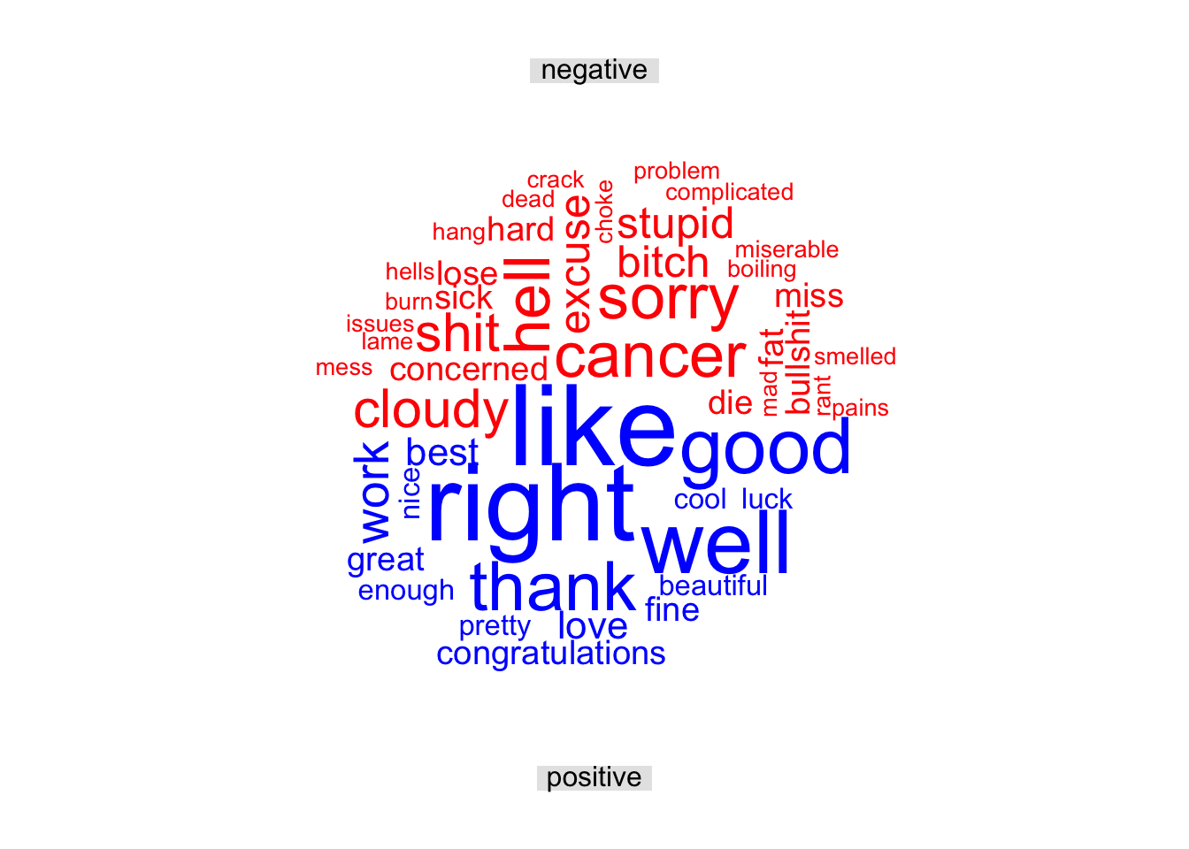
I generated wordcloud using the bing sentiment analysis, which categorizes words into positive and negative groups. From the word cloud, we can see that the episode contains a number of negative words, but also some positive ones like “good,” “like,” and “beautiful.” But also we need to consider that these words are analyzed in isolation. While they are labeled as positive or negative by default, their actual meaning can change depending on the context in which they’re used.
bing <- my_data_txt %>% unnest_tokens(word, text) %>%
  inner_join(get_sentiments("bing")) %>%
  count(word, sentiment, sort = TRUE)

bing %>% slice(1:10)
word sentiment n
1 like positive 20
2 right positive 19
3 well positive 15
4 good positive 13
5 thank positive 11
6 work positive 7
7 best positive 5
8 cancer negative 5
9 hell negative 5
10 love positive 5From the list above, we can see top 10 words that made the biggest sentiment contributions. Among these, 2 words are negative (“cancer”, “hell”) while the rest are positive. By looking at the result, the overall tone of the episode can be more positive. However, the appeareance of word “cancer” can mean that probably one of the characters have illness, which introduces a more emotionally heavy or serious atmosphere. Similarly, the word “hell” often reflects anger, frustration, or a chaotic situation. These two words hint at deeper emotional layers while other words gives more positive emotions.
# afinn <- my_data_txt %>% unnest_tokens(word, text) %>%
#   inner_join(get_sentiments("afinn")) %>%
#   count(word, value, sort = TRUE) %>%
#   mutate(contribution = n*value)

# afinn %>% arrange(contribution) %>% slice(1:3)

# afinn %>% arrange(desc(contribution)) %>% slice(1:3)
Three worst words are “no”, “hell”, “shit”.
Three best words are “like”, “good”, “thank”.
# sum(afinn$contribution)Sum of values is positive 146.
The sum of sentiment values can help identify the overall emotional tone of an episode. In our case, since the total score is positive, it suggests the episode is generally positive. However, by analyzing in this way we are missing true meaning of words. For example, the word “hell” might be used in a positive or humorous way, while words considered positive—like “great”—could be used sarcastically, meaning the opposite. Additionally, simply counting the frequency of words overlooks deeper meaning. The tone and impact of a word can depend on who said it, how it was said, and in what scene. Without that context, the analysis can be incomplete or even misleading.