library(tidyverse)
library(dplyr)
library(lubridate)
library(leaflet)

vancouver_df <- read.csv('./vancouver_311_requests.csv', sep = ';')City service requests made in Vancouver, British Columbia from 2022 to the present.
This project focuses on exploring and visualizing data related to city service requests in Vancouver, British Columbia. The dataset is sourced from Vancouver’s Open Data Portal and contains information about service requests made from 2022 to the present.
This work is part of an assignment for the AD699 Data Mining course.
Data Exploration
str() function shows structure of an object. From the result below we can see that, type of our dataset is data.frame which consists of 842862 rows and 13 columns. And also shows the type of each column.
str(vancouver_df)'data.frame': 842862 obs. of 13 variables:
$ Department : chr "ENG - Parking Enforcement and Operations" "FSC - Property Tax" "DBL - Services Centre" "DBL - Services Centre" ...
$ Service.request.type : chr "Abandoned or Uninsured Vehicle Case" "Property Tax Request Case" "Building and Development Inquiry Case" "Building and Development Inquiry Case" ...
$ Status : chr "Close" "Close" "Close" "Close" ...
$ Closure.reason : chr "Insufficient info" "Alternate Service Required" "Service provided" "Service provided" ...
$ Service.request.open.timestamp: chr "2023-10-24T16:38:00-04:00" "2023-10-24T16:40:00-04:00" "2023-10-24T16:42:00-04:00" "2023-10-24T16:45:00-04:00" ...
$ Service.request.close.date : chr "2023-10-24" "2023-10-25" "2023-10-27" "2023-10-27" ...
$ Last.modified.timestamp : chr "2023-10-24T18:58:39-04:00" "2023-10-25T14:05:13-04:00" "2023-10-27T17:09:55-04:00" "2023-10-27T15:05:34-04:00" ...
$ Address : chr "" "" "" "" ...
$ Local.area : chr "" "Fairview" "Downtown" "Arbutus Ridge" ...
$ Channel : chr "Mobile App" "Phone" "WEB" "WEB" ...
$ Latitude : num NA NA NA NA NA ...
$ Longitude : num NA NA NA NA NA ...
$ geom : chr "" "" "" "" ...In our dataset 23 unique values of Local.area including empty value.
unique(vancouver_df$Local.area) [1] "" "Fairview"
[3] "Downtown" "Arbutus Ridge"
[5] "Strathcona" "Mount Pleasant"
[7] "Shaughnessy" "West Point Grey"
[9] "Kitsilano" "West End"
[11] "Sunset" "South Cambie"
[13] "Marpole" "Kensington-Cedar Cottage"
[15] "Grandview-Woodland" "Oakridge"
[17] "Hastings-Sunrise" "Renfrew-Collingwood"
[19] "Riley Park" "Victoria-Fraserview"
[21] "Kerrisdale" "Killarney"
[23] "Dunbar-Southlands" length(unique(vancouver_df$Local.area))[1] 23sunset_df <- filter(vancouver_df, Local.area == 'Sunset')
nrow(sunset_df)[1] 33036Now I have 33036 records from my area Sunset.
str(sunset_df)'data.frame': 33036 obs. of 13 variables:
$ Department : chr "DBL - Services Centre" "DBL - Animal Services" "DBL - Services Centre" "DBL - Property Use Inspections" ...
$ Service.request.type : chr "Building and Development Inquiry Case" "Animal Concern Case" "Building and Development Inquiry Case" "Private Property Concern Case" ...
$ Status : chr "Close" "Close" "Close" "Close" ...
$ Closure.reason : chr "Service provided" "Further action has been planned" "Service provided" "Assigned to inspector" ...
$ Service.request.open.timestamp: chr "2023-10-24T18:05:19-04:00" "2023-10-24T20:05:27-04:00" "2023-08-13T14:02:01-04:00" "2023-08-13T22:54:01-04:00" ...
$ Service.request.close.date : chr "2023-10-25" "2023-10-24" "2023-08-16" "2023-08-16" ...
$ Last.modified.timestamp : chr "2023-10-25T14:20:17-04:00" "2023-10-24T20:33:26-04:00" "2023-08-16T13:46:59-04:00" "2023-08-16T15:01:47-04:00" ...
$ Address : chr "" "" "" "" ...
$ Local.area : chr "Sunset" "Sunset" "Sunset" "Sunset" ...
$ Channel : chr "WEB" "Phone" "WEB" "WEB" ...
$ Latitude : num NA NA NA NA NA ...
$ Longitude : num NA NA NA NA NA ...
$ geom : chr "" "" "" "" ...The following columns have date-related information: Service.request.open.timestamp, Service.request.close.date, Last.modified.timestamp. Now R see them as character not date.
sunset_df$Service.request.open.timestamp <- as.Date(sunset_df$Service.request.open.timestamp)
sunset_df$Service.request.close.date <- as.Date(sunset_df$Service.request.close.date)
sunset_df$Last.modified.timestamp <- as.Date(sunset_df$Last.modified.timestamp)

str(sunset_df)
'data.frame': 33036 obs. of 13 variables:
$ Department : chr "DBL - Services Centre" "DBL - Animal Services" "DBL - Services Centre" "DBL - Property Use Inspections" ...
$ Service.request.type : chr "Building and Development Inquiry Case" "Animal Concern Case" "Building and Development Inquiry Case" "Private Property Concern Case" ...
$ Status : chr "Close" "Close" "Close" "Close" ...
$ Closure.reason : chr "Service provided" "Further action has been planned" "Service provided" "Assigned to inspector" ...
$ Service.request.open.timestamp: Date, format: "2023-10-24" "2023-10-24" ...
$ Service.request.close.date : Date, format: "2023-10-25" "2023-10-24" ...
$ Last.modified.timestamp : Date, format: "2023-10-25" "2023-10-24" ...
$ Address : chr "" "" "" "" ...
$ Local.area : chr "Sunset" "Sunset" "Sunset" "Sunset" ...
$ Channel : chr "WEB" "Phone" "WEB" "WEB" ...
$ Latitude : num NA NA NA NA NA ...
$ Longitude : num NA NA NA NA NA ...
$ geom : chr "" "" "" "" ...Now R sees these columns as Date.
sunset_df <- sunset_df %>% mutate(duration = as.numeric(Service.request.close.date - Service.request.open.timestamp, units="days"))To extract numeric value of difference between dates, I used as.numeric() function and specified units as days.
sum(is.na(sunset_df))[1] 41170In our dataset 41170 total NA values.
colSums(is.na(sunset_df)) Department Service.request.type
0 0
Status Closure.reason
0 0
Service.request.open.timestamp Service.request.close.date
0 523
Last.modified.timestamp Address
0 0
Local.area Channel
0 0
Latitude Longitude
20062 20062
geom duration
0 523 Here is the total # of NA values for each column. The columns Latitude and Longitude each has 20062 missing values, probably Address column is also contain empty values. The service close date didn’t recorded 523 times, which is affected duration column too.
birthday_reqs <- sunset_df %>% filter(month(Service.request.open.timestamp) == 11 & day(Service.request.open.timestamp) == 24)
nrow(birthday_reqs)
[1] 64My birthday is in November 24th, and by using functions from lubridate package, we see that in my birthday occurred 64 requests.
birthday_reqs_channel <- birthday_reqs %>% group_by(Channel) %>% summarise(Count = n()) %>% arrange(desc(Count))
birthday_reqs_channel
# A tibble: 4 × 2
Channel Count
<chr> <int>
1 WEB 27
2 Phone 25
3 Mobile App 11
4 Chat 1On this date the most of requests came from WEB, Phone channels.
birthday_reqs_types <- birthday_reqs %>% group_by(Service.request.type) %>% summarise(Count = n()) %>% arrange(desc(Count))
birthday_reqs_types
# A tibble: 31 × 2
Service.request.type Count
<chr> <int>
1 Missed Green Bin Pickup Case 9
2 Green Bin Request Case 7
3 Abandoned Non-Recyclables-Small Case 6
4 Business Licence Request Case 5
5 Abandoned or Uninsured Vehicle Case 4
6 Building and Development Inquiry Case 4
7 Abandoned Recyclables Case 2
8 Sewer Drainage and Design Inquiry Case 2
9 Street Light Out Case 2
10 Street Light Pole Maintenance Case 2
# ℹ 21 more rowsThe top 5 requests inlcude cases related to Green bin (total 16), non-recyclables(total 6), business licence and abandoned vehicle.
sunset_df %>% group_by(Year = year(Service.request.open.timestamp)) %>% summarise(Count = n())# A tibble: 4 × 2
Year Count
<dbl> <int>
1 2022 10840
2 2023 10192
3 2024 11018
4 2025 986The dataset only contains city service requests going through January of 2025, so the 2025 annual total is not really comparable to the numbers from other years.
sunset_df %>% group_by(Channel) %>% summarise(avg = mean(duration, na.rm = TRUE)) %>% arrange(desc(avg))# A tibble: 7 × 2
Channel avg
<chr> <dbl>
1 E-mail 10.5
2 Chat 10.1
3 Mobile App 10.1
4 Phone 9.85
5 WEB 9.39
6 Social Media 6.64
7 Mail 3 For the channels like E-mail, Chat, Mobile App the average duration to complete service request is more than 10 days. On the other hand, by using Mail channel they spent 3 days on average. Perhaps, since nowadays a lot of requests came from digital/web apps, and the older requests can left at the bottom of the queue which can lead to delays to finish them. Also, different types of requests can be sent through each type of channel, more complicated use E-mail, and small cases use Mail. Or some other factor can affect.
open_reqs <- sunset_df %>% filter(Status == "Open")
# nrow(open_reqs)
open_reqs %>% group_by(Month = month(Service.request.open.timestamp)) %>% summarise(Count = n())
# A tibble: 12 × 2
Month Count
<dbl> <int>
1 1 272
2 2 16
3 3 14
4 4 19
5 5 21
6 6 23
7 7 25
8 8 28
9 9 10
10 10 29
11 11 30
12 12 36272 out of 523 total open requests are in January only. The dataset was retrieved in January 2025, and most of the yet-unresolved cases in it are recent ones – that’s what explains the January bump
names(sunset_df) [1] "Department" "Service.request.type"
[3] "Status" "Closure.reason"
[5] "Service.request.open.timestamp" "Service.request.close.date"
[7] "Last.modified.timestamp" "Address"
[9] "Local.area" "Channel"
[11] "Latitude" "Longitude"
[13] "geom" "duration" sunset_df <- sunset_df %>% rename(Service.request.open.date = Service.request.open.timestamp)
names(sunset_df) [1] "Department" "Service.request.type"
[3] "Status" "Closure.reason"
[5] "Service.request.open.date" "Service.request.close.date"
[7] "Last.modified.timestamp" "Address"
[9] "Local.area" "Channel"
[11] "Latitude" "Longitude"
[13] "geom" "duration" I renamed the column Service.request.open.timestamp to Service.request.open.date, because now it contains only dates without time.
sunset_df$Address <- NULL

names(sunset_df)
[1] "Department" "Service.request.type"
[3] "Status" "Closure.reason"
[5] "Service.request.open.date" "Service.request.close.date"
[7] "Last.modified.timestamp" "Local.area"
[9] "Channel" "Latitude"
[11] "Longitude" "geom"
[13] "duration" Now our dataset has 13 columns.
Data Visualization
data1 <- sunset_df %>%
  group_by(DayOfWeek = wday(Service.request.open.date, label = TRUE)) %>%
  summarise(Count = n()) %>%
  mutate(DayOfWeek = factor(DayOfWeek, levels = c("Mon", "Tue", "Wed", "Thu", "Fri", "Sat", "Sun"), ordered = TRUE)) %>%
  arrange(DayOfWeek)

library(ggplot2)
library(ggthemes)

ggplot(data1, aes(x=DayOfWeek, y=Count)) +
  geom_bar(stat = "identity", fill="thistle", color="black") +
  labs(title = "City Service requests by Day of Week",
       x = "Day of Week",
       y = "Number of Requests") +
  theme_clean()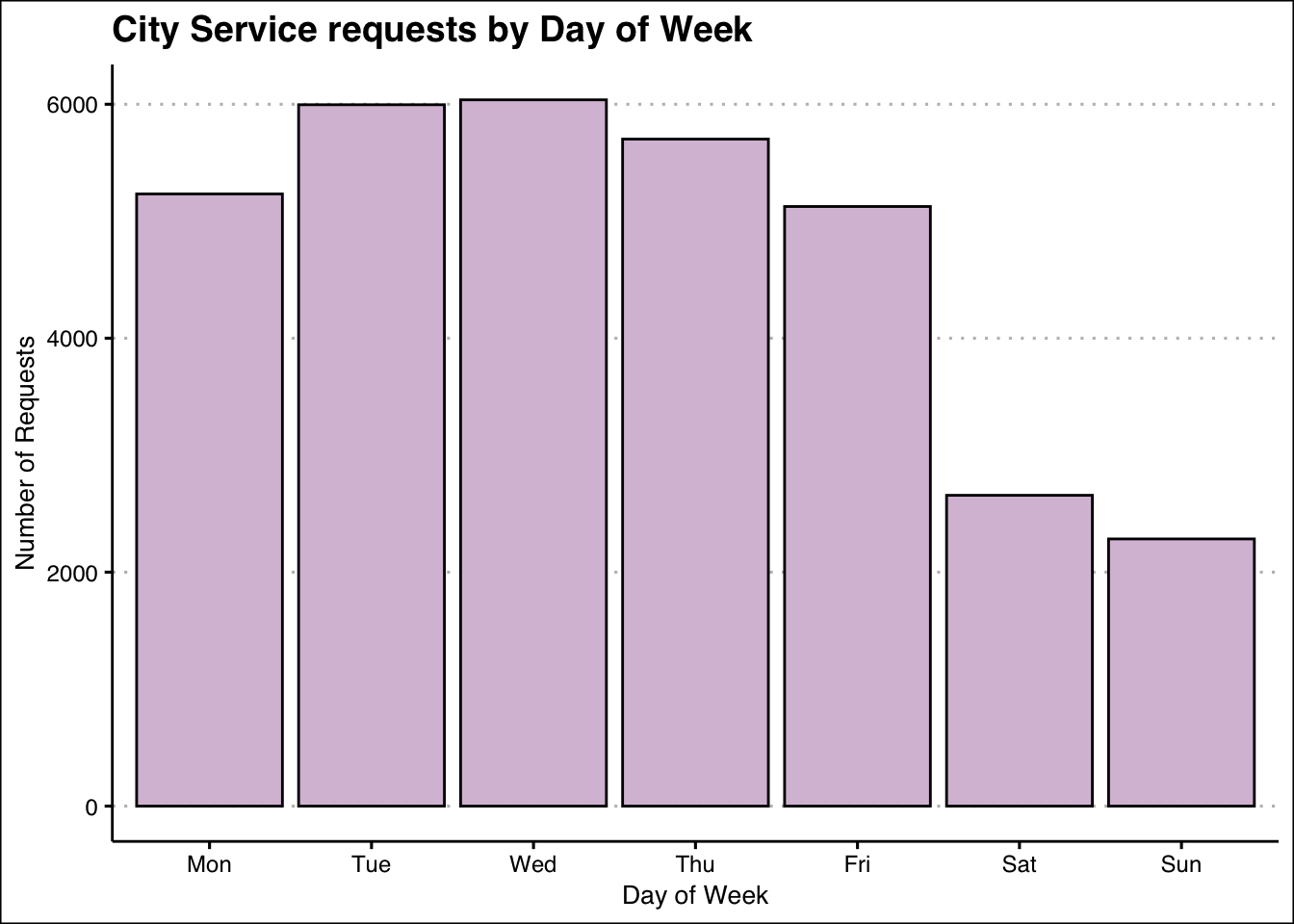
The bar chart displays how many requests were made each day of week.Weekends have only about half the volume of requests, and the middle of the week is when the highest number of requests are occur. Maybe in the weekdays people tend to have more time or prefer to report rather than on weekends.
top7_req_types <- sunset_df %>% group_by(Service.request.type) %>% summarise(Count = n()) %>% arrange(desc(Count)) %>% slice_head(n=7)
top7_req_types$Service.request.type
[1] "Missed Green Bin Pickup Case"
[2] "Building and Development Inquiry Case"
[3] "Missed Garbage Bin Pickup Case"
[4] "Garbage Bin Request Case"
[5] "City and Park Trees Maintenance Case"
[6] "Green Bin Request Case"
[7] "Abandoned Non-Recyclables-Small Case" sunset_df_top7 <- sunset_df %>% filter(Service.request.type %in% top7_req_types$Service.request.type)
nrow(sunset_df_top7)[1] 16088Now there are only 16088 records with top 7 service request types.
data2 <- sunset_df_top7 %>%
  group_by(DayOfWeek = wday(Service.request.open.date, label = TRUE), Department) %>%
  summarise(Count = n(), .groups = "drop") %>%
  mutate(DayOfWeek = factor(DayOfWeek, levels = c("Mon", "Tue", "Wed", "Thu", "Fri", "Sat", "Sun"), ordered = TRUE)) %>%
arrange(DayOfWeek)ggplot(data2, aes(x=DayOfWeek, y=Count, fill = Department)) +
geom_bar(stat = "identity", position = "dodge") +
scale_fill_manual(values = c("#E69F00", "#56B4E9", "#009E73")) +
labs(title = "City Service requests by Day of Week and Department",
x = "Day of Week",
y = "Number of Requests") +
theme_foundation()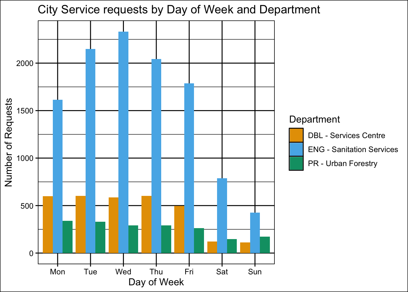
The main part of service requests from “ENG-Sanitation Services” no matter which day is it. The “PR-Urban Forestry” requests stays the same during the days of week, while “DBL-Services Centre” requests drops significantly on weekends. What if DBL Services Centre offices are closed on weekends, so citizens know this and wait until the week to make the reports? But if Urban Forestry is set up differently, that might explain why it doesn’t show such a big change. Or maybe Urban Forestry requests can be depend on weather conditions, and occur not so often like Sanitation services.
data3 <- sunset_df_top7 %>% group_by(Month = month(Service.request.open.date, label = TRUE), Service.request.type) %>%
  summarise(Count = n(), .groups = "drop")

ggplot(data3, aes(x=Month, y=Count, fill = Service.request.type)) +
  geom_bar(stat = "identity") +
  labs(title = "City Service requests by Month and Service Request Type",
       x = "Month",
       y = "Number of Requests") +
  theme_calc()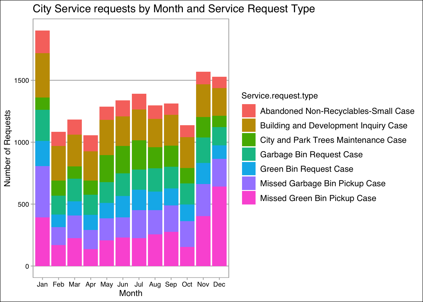
January has highest number of requests, followed by November and December. Missed Green Bin Pickup Case occurred in these 3 months more than other months. In January post-holiday waste can put extra pressure to collection system. Also, November and December which are holiday season can lead to increase of waste too. November is often peak time for leaf fall, it can also impact collection system. It’s interesting that Building and Development inquires spike in January, and stays high during the year. January is like a month of new beginnings, when people tend to start new projects. Maybe it can be one of the reasons of large number of requests.
ggplot(sunset_df_top7, aes(x=duration)) +
  geom_histogram(binwidth = 50, fill = "skyblue", color = "black", boundary = 0) +
  labs(title = "Distribution of Service Request Duration",
       x = "Duration (in days)",
       y = "Number of Requests"
       ) +
  theme_bw()
Warning: Removed 236 rows containing non-finite outside the scale range
(`stat_bin()`).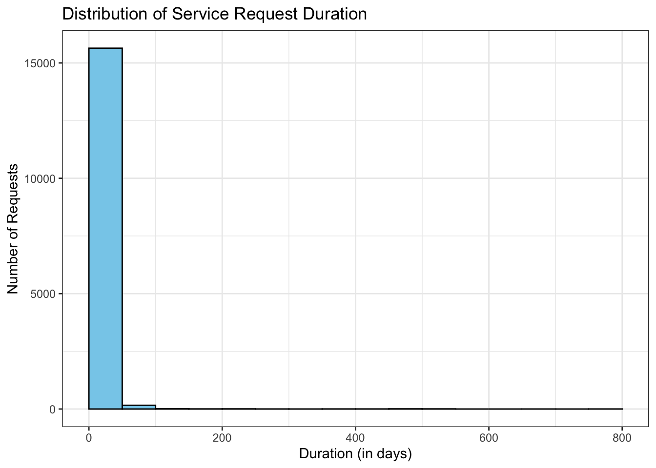
The distribution is left-skewed. It’s interesting that for some requests to be closed took around 800 days, maybe it’s result of some technical issues, or these cases delayed because of legal issues. And in most cases to complete request took between 0 to 50 days. By setting binwidth = 50, I say that each bin represents 50 days.
ggplot(sunset_df_top7, aes(x=duration)) +
  geom_histogram(binwidth = 30, fill = "skyblue", color = "black", boundary = 0) +
  facet_wrap(~Service.request.type) +
  labs(title = "Distribution of Service Request Duration",
       x = "Duration (in days)",
       y = "Number of Requests"
       ) +
  theme_bw()
Warning: Removed 236 rows containing non-finite outside the scale range
(`stat_bin()`).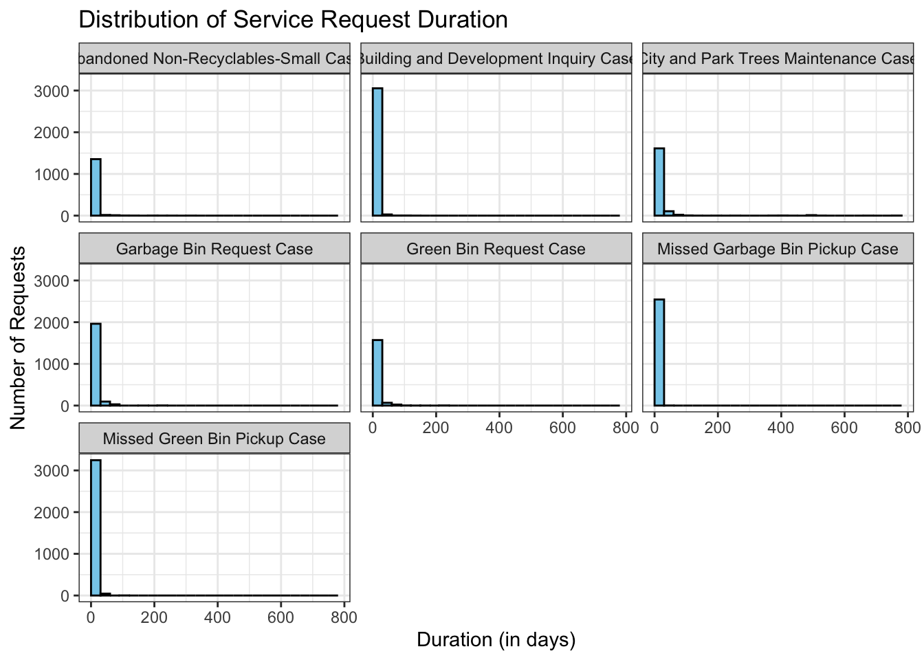
Most of the city requests have a same pattern, which can represent that city requests processes in a quick turnaround time. In some cases it can take longer than 30 days, maybe because of legal issues which can occur for the City and Trees Maintenance case (permits to make changes from multiple departments)
ggplot(sunset_df_top7, aes(x=Channel, fill = Service.request.type)) +
  geom_bar(position = "fill") +
  labs(title = "Distribution of Service Request Type by Channel",
       y = "Proportion of requests",
       fill = "Service Request Type")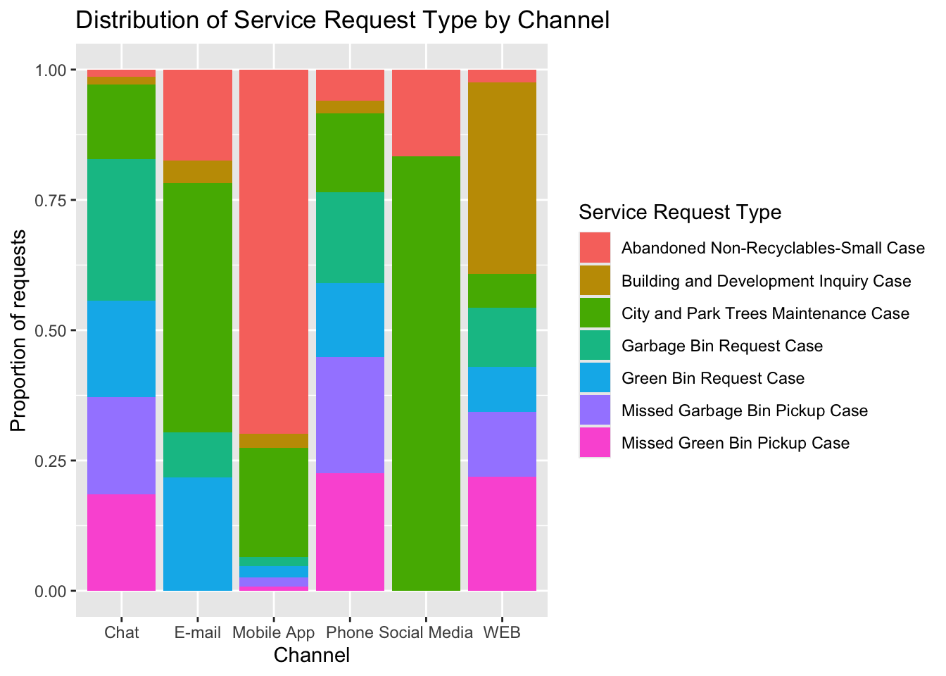
This plot shows the distribution of service request types across channels. Interesting, that Abandoned Non-Recyclables mostly reported via mobile app, while City and Park Maintenance dominate in Social Media and E-mail. Also, Building and Development Inquiry mostly reported via WEB. Different requests seems like have preferred channels. For instance, garbage and green bin requests prefer chat or phone, that do not require any additional resources like images. For the City and Park Maintenance social media is popular, maybe because people prefer post about their awareness of city to public discussion.
Created map with Esri World Imagery tiles, and added popup text which will display department name for each service request.
sunset_df_map <- sunset_df %>% filter(!is.na(Latitude) & !is.na(Longitude))

leaflet(data = sunset_df_map) %>%
  addTiles() %>%
addCircles(~Longitude, ~Latitude)leaflet(data = sunset_df_map) %>%
addProviderTiles("Esri.WorldImagery") %>%
addCircles(~Longitude, ~Latitude, radius = 5, color = "gold", popup = ~Department)