library(tidyverse)
library(dplyr)
library(caret)
library(rpart)
library(rpart.plot)

vg <- read.csv('vgchartz-2024.csv')Classification Tree
Developed a classification model to predict video game sales performance using a real-world video game dataset. Preprocessed the data through binning, factor conversion, and top-category filtering. Built, visualized, and pruned decision trees using cross-validation, and evaluated model performance using confusion matrices.
This work is part of an assignment for the AD699 Data Mining course.
This dataset appears to contain information about video games, including the title, the console it was developed for, genre, publisher, developer, game rating, various sales numbers, release date, and, if available, the last update date. While some titles appear multiple times, other variables indicate that these entries correspond to the same game released on different consoles or different versions, such as remakes. The critic_score represents the overall rating of a game, with a maximum score of 10. And the dataset includes sales data across different regions (NA, JP, PAL, Other), and difference between numbers suggest the game popularity across various geographical areas. Furthermore, there is huge number of NAs.
After using equal frequency binning method to our output variable, we can see that the data equally was distributed within three groups: Low, Medium, High.
vg$total_sales <- cut(vg$total_sales,
                      breaks = quantile(vg$total_sales, probs = seq(0, 1, length.out = 4), na.rm = TRUE),
                      include.lowest = TRUE,
                      labels = c("Low", "Medium", "High"))
table(vg$total_sales)
   Low Medium   High
6339 6386 6197 str(vg)'data.frame': 64016 obs. of 14 variables:
$ img : chr "/games/boxart/full_6510540AmericaFrontccc.jpg" "/games/boxart/full_5563178AmericaFrontccc.jpg" "/games/boxart/827563ccc.jpg" "/games/boxart/full_9218923AmericaFrontccc.jpg" ...
$ title : chr "Grand Theft Auto V" "Grand Theft Auto V" "Grand Theft Auto: Vice City" "Grand Theft Auto V" ...
$ console : chr "PS3" "PS4" "PS2" "X360" ...
$ genre : chr "Action" "Action" "Action" "Action" ...
$ publisher : chr "Rockstar Games" "Rockstar Games" "Rockstar Games" "Rockstar Games" ...
$ developer : chr "Rockstar North" "Rockstar North" "Rockstar North" "Rockstar North" ...
$ critic_score: num 9.4 9.7 9.6 NA 8.1 8.7 8.8 9.8 8.4 8 ...
$ total_sales : Factor w/ 3 levels "Low","Medium",..: 3 3 3 3 3 3 3 3 3 3 ...
$ na_sales : num 6.37 6.06 8.41 9.06 6.18 9.07 9.76 5.26 8.27 4.99 ...
$ jp_sales : num 0.99 0.6 0.47 0.06 0.41 0.13 0.11 0.21 0.07 0.65 ...
$ pal_sales : num 9.85 9.71 5.49 5.33 6.05 4.29 3.73 6.21 4.32 5.88 ...
$ other_sales : num 3.12 3.02 1.78 1.42 2.44 1.33 1.14 2.26 1.2 2.28 ...
$ release_date: chr "2013-09-17" "2014-11-18" "2002-10-28" "2013-09-17" ...
$ last_update : chr "" "2018-01-03" "" "" ...vg$img <- as.factor(vg$img)
vg$title <- as.factor(vg$title)
vg$console <- as.factor(vg$console)
vg$genre <- as.factor(vg$genre)
vg$publisher <- as.factor(vg$publisher)
vg$developer <- as.factor(vg$developer)
vg$release_date <- as.factor(vg$release_date)
vg$last_update <- as.factor(vg$last_update)
str(vg)'data.frame': 64016 obs. of 14 variables:
$ img : Factor w/ 56177 levels "/games/boxart/1000386ccc.jpg",..: 31526 27433 6702 42887 25079 47407 47389 23589 12344 23571 ...
$ title : Factor w/ 39798 levels "_summer ##","- Arcane preRaise -",..: 13767 13767 13779 13767 5281 5291 5276 27100 5283 5283 ...
$ console : Factor w/ 81 levels "2600","3DO","3DS",..: 57 58 56 76 58 76 76 58 76 57 ...
$ genre : Factor w/ 20 levels "Action","Action-Adventure",..: 1 1 1 1 16 16 16 2 16 16 ...
$ publisher : Factor w/ 3383 levels "][ Games","@unepic_fran",..: 2514 2514 2514 2514 84 84 84 2514 84 84 ...
$ developer : Factor w/ 8863 levels "",".theprodukkt",..: 6580 6580 6580 6580 8072 3787 8072 6576 8072 8072 ...
$ critic_score: num 9.4 9.7 9.6 NA 8.1 8.7 8.8 9.8 8.4 8 ...
$ total_sales : Factor w/ 3 levels "Low","Medium",..: 3 3 3 3 3 3 3 3 3 3 ...
$ na_sales : num 6.37 6.06 8.41 9.06 6.18 9.07 9.76 5.26 8.27 4.99 ...
$ jp_sales : num 0.99 0.6 0.47 0.06 0.41 0.13 0.11 0.21 0.07 0.65 ...
$ pal_sales : num 9.85 9.71 5.49 5.33 6.05 4.29 3.73 6.21 4.32 5.88 ...
$ other_sales : num 3.12 3.02 1.78 1.42 2.44 1.33 1.14 2.26 1.2 2.28 ...
$ release_date: Factor w/ 7923 levels "","1971-12-03",..: 6007 6357 2845 6007 6573 5506 5197 7244 5769 5769 ...
$ last_update : Factor w/ 1546 levels "","2017-11-28",..: 1 15 1 1 26 1 1 285 109 109 ...After converting all chr parameters to factor, our dataset contains only numbers or factors.
Next we are going to do some “topN” filtering.
top_7_Console <- vg %>%
  count(console, sort = TRUE) %>%
  slice(1:7)
top_7_Console
console n
1 PC 12617
2 PS2 3565
3 DS 3288
4 PS4 2878
5 PS 2707
6 NS 2337
7 XBL 21207 popular console types: PC, PS2, DS, PS4, PS, NS, XBL. Also there is huge difference between PC and other remaining values, making PC much more popular. This is likely due to its open system, allowing users to install and download games freely without strict platform restrictions.
top_7_Genre <- vg %>%
  count(genre, sort = TRUE) %>%
  slice(1:7)
top_7_Genre
genre n
1 Misc 9304
2 Action 8557
3 Adventure 6260
4 Role-Playing 5721
5 Sports 5586
6 Shooter 5410
7 Platform 40017 most common genres: misc, action, adventure, role-playing, sports, shooter, platform. The most prevalent genre is Miscellaneous, likely due to games that don’t fit into traditional categories or are poorly documented. Following that, Action games are the second most popular, with Adventure games ranking third. The popularity of platform games (Mario, Zelda or Sonic) shows that traditional gameplay styles still have a strong place in market.
top_7_Publisher <- vg %>%
  count(publisher, sort = TRUE) %>%
  slice(1:7)
top_7_Publisher
publisher n
1 Unknown 8842
2 Sega 2207
3 Ubisoft 1663
4 Electronic Arts 1619
5 Activision 1582
6 Konami 1544
7 Nintendo 14767 most common publishers: unknown, sega, ubisoft, electronic arts, activision, konami, nintendo. Notably, 8,842 records lack publisher information, categorized under “Unknown.” Among named publishers, Sega remains a key player. Also, Ubisoft, EA, Activision have released most of the popular games over the last few years.
top_7_Developer <- vg %>%
  count(developer, sort = TRUE) %>%
  slice(1:7)
top_7_Developer
developer n
1 Unknown 4435
2 Konami 976
3 Sega 915
4 Capcom 870
5 Namco 489
6 Square Enix 425
7 SNK Corporation 4087 most common developers: unknown, konami, sega, namco, square enix, capcom, snk corporation. Similarly, 4,435 records lack developer information. Several major developers, such as Sega and Konami, also appear among the top publishers, reinforcing their influence in the industry.
vg <- vg %>% filter(console %in% top_7_Console$console &
                      genre %in% top_7_Genre$genre &
                      publisher %in% top_7_Publisher$publisher &
                      developer %in% top_7_Developer$developer)

nrow(vg)
[1] 939After applying these filters, the dataset is reduced to 939 rows.
vg <- droplevels(vg)
nrow(vg)
[1] 939The dataset contains 939 records.
set.seed(79)
vg.index <- sample(c(1:nrow(vg)), nrow(vg)*0.6)
vg_train <- vg[vg.index, ]
vg_valid <- vg[-vg.index, ]
Next we will use rpart.plot to display a classification tree that depicts our model.
model <- rpart(total_sales ~ console + genre + publisher + developer + critic_score, method = 'class', data = vg_train)

rpart.plot(model)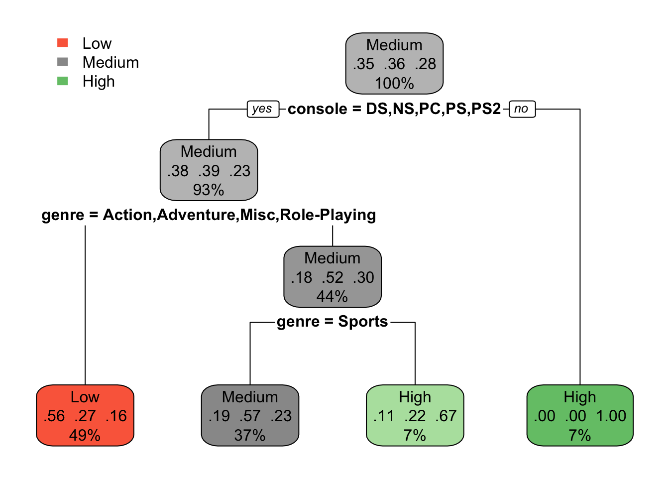
The initial plot starts with default parameters, where the tree starts from console varaible at the root. Each node represents type of total_sales (Low, Medium, High) differentiated by color. Within each node, we see class probabilities and the percentage of observations classified at that node.
rpart.plot(model, extra=2, fallen.leaves = FALSE)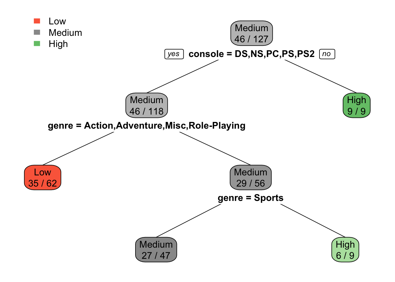
After adding extra=2, in the new plot the class rate is relative to the total number of observations in each class. For instance, in the second left node, 50 observations belong to Low sales category out of 102 total observations. And setting fallen.leaves = FALSE, moves the leaf nodes away from the bottom, changing the structure of trees.
rpart.plot(model, type=5, extra = 2, fallen.leaves=FALSE)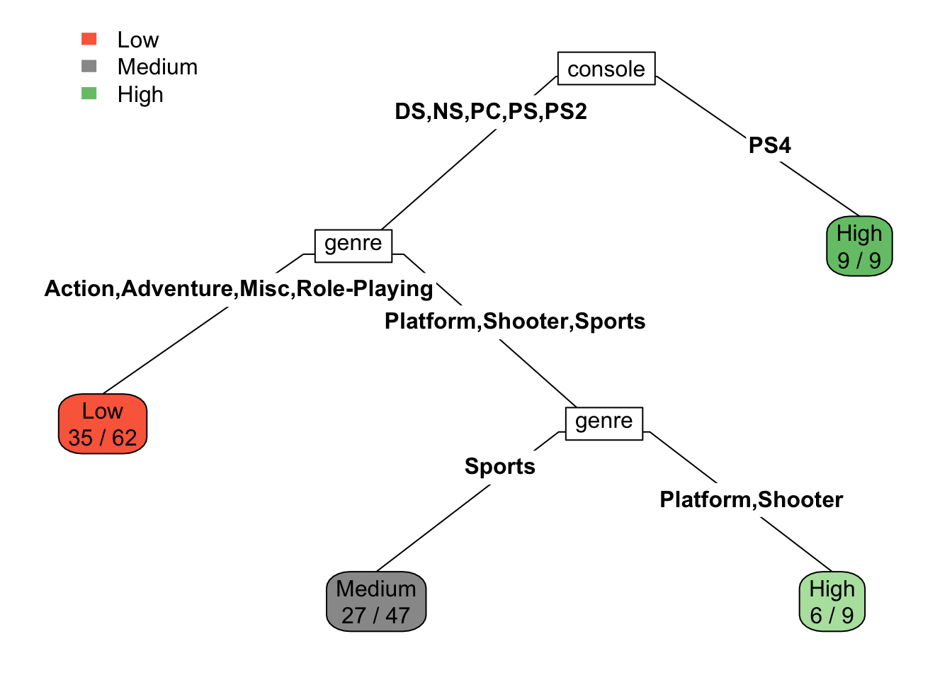
In the third plot used type=5, which adds variable names for each split line, and class labels appear only at the leaves. This layout more intuitive, as it avoids overwhelming details such as numbers and labels.
The root node is console variable, and rule is Console = DS or PC. The root node is starting point of model, and have highest impact on outcome variable. In our model, the type of console is primary factor to decide total sales number. So, this approach can help strategize future plans for the game publisher, focusing more on high-performance consoles.
We see that from 5 input variables (console, genre, publisher, developer, critic score), only 2 (console, genre) appears in the tree model, as a useful parameters to predict price. Variable subset selection is automatic since it is part of the split selection.
rpart.rules(model) total_sales Low Medi High
Low [ .56 .27 .16] when console is DS or NS or PC or PS or PS2 & genre is Action or Adventure or Misc or Role-Playing
Medium [ .19 .57 .23] when console is DS or NS or PC or PS or PS2 & genre is Sports
High [ .11 .22 .67] when console is DS or NS or PC or PS or PS2 & genre is Platform or Shooter
High [ .00 .00 1.00] when console is PS4 From the rules of our model, let’s describe second rule (index = 10): The video game is for PS console and Sports genre, by following tree nodes this game will be classified into Medium sales group.
complex_model <- rpart(total_sales ~ console + genre + publisher + developer + critic_score, method="class", cp=0, minsplit=2, data = vg_train)

rpart.plot(complex_model, extra=1, fallen.leaves=FALSE)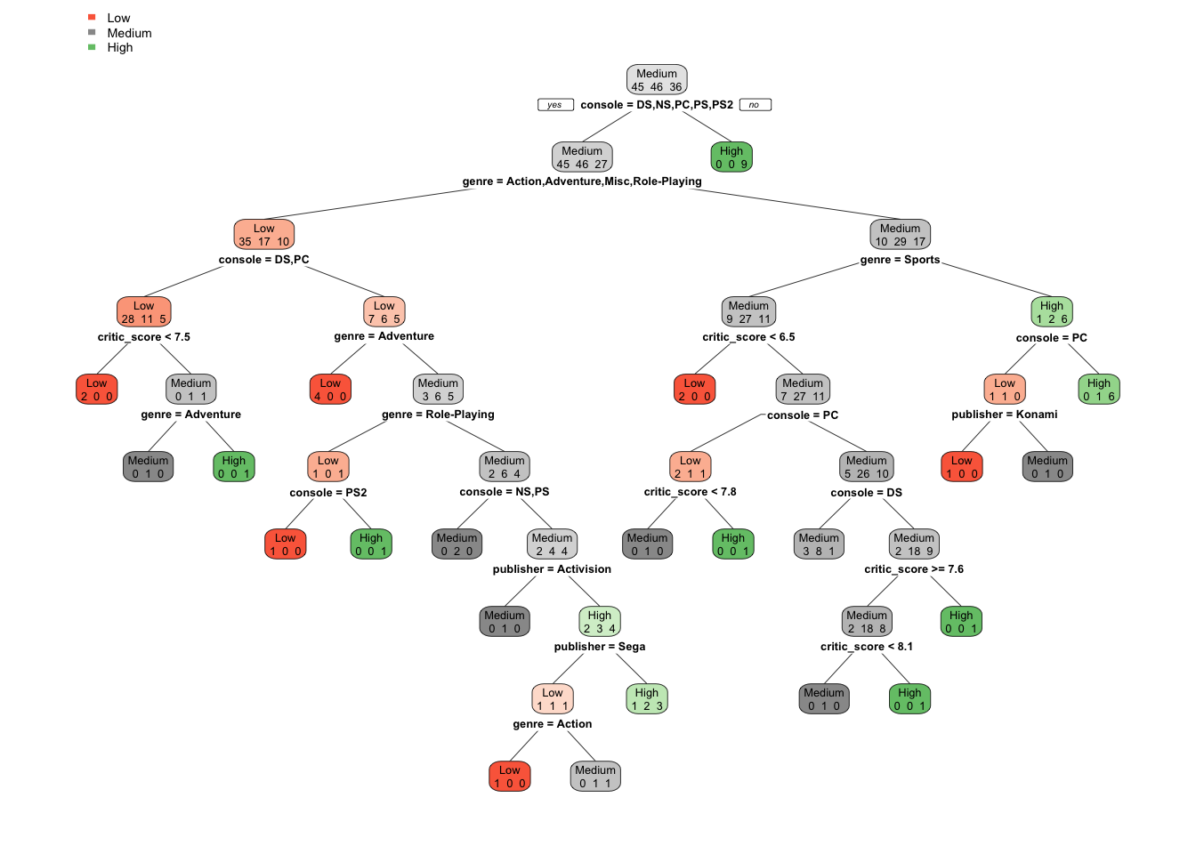
five_fold_cv <- rpart(total_sales ~ console + genre + publisher + developer + critic_score, method="class",
                      cp=0.00001, minsplit=5, xval=5, data=vg_train)

a <- printcp(five_fold_cv)
Classification tree:
rpart(formula = total_sales ~ console + genre + publisher + developer +
    critic_score, data = vg_train, method = "class", cp = 1e-05,
    minsplit = 5, xval = 5)

Variables actually used in tree construction:
[1] console      critic_score genre

Root node error: 81/127 = 0.6378

n=127 (436 observations deleted due to missingness)

         CP nsplit rel error  xerror     xstd
1 0.1666667      0   1.00000 1.08642 0.064178
2 0.0925926      2   0.66667 0.85185 0.069303
3 0.0493827      4   0.48148 0.85185 0.069303
4 0.0370370      5   0.43210 0.77778 0.069562
5 0.0246914      6   0.39506 0.76543 0.069545
6 0.0123457      7   0.37037 0.77778 0.069562
7 0.0061728     10   0.33333 0.77778 0.069562
8 0.0000100     12   0.32099 0.80247 0.069545
a <- data.frame(a)
a CP nsplit rel.error xerror xstd
1 0.16666667 0 1.0000000 1.0864198 0.06417809
2 0.09259259 2 0.6666667 0.8518519 0.06930294
3 0.04938272 4 0.4814815 0.8518519 0.06930294
4 0.03703704 5 0.4320988 0.7777778 0.06956221
5 0.02469136 6 0.3950617 0.7654321 0.06954496
6 0.01234568 7 0.3703704 0.7777778 0.06956221
7 0.00617284 10 0.3333333 0.7777778 0.06956221
8 0.00001000 12 0.3209877 0.8024691 0.06954496From the complexity parameter table for eight trees, we see that xerror value decreased at some point and started to increase again. This minimum value of cross validation error (0.7037037) gives optimal cp value. In our case cp = 0.03703704
pruned.ct <- prune(five_fold_cv,
                   cp=five_fold_cv$cptable[which.min(five_fold_cv$cptable[,"xerror"]),"CP"])

rpart.plot(pruned.ct,type=5, extra = 2, fallen.leaves=FALSE)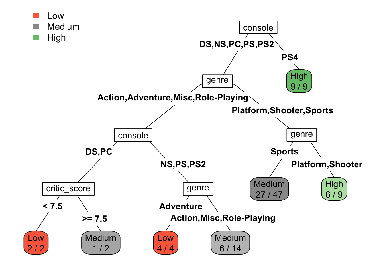
# Huge tree results
complex_model.pred <- predict(complex_model, vg_train, type="class")
confusionMatrix(complex_model.pred, vg_train$total_sales)
Confusion Matrix and Statistics
Reference
Prediction Low Medium High
Low 39 10 4
Medium 5 33 9
High 1 3 23
Overall Statistics
Accuracy : 0.748
95% CI : (0.6633, 0.8208)
No Information Rate : 0.3622
P-Value [Acc > NIR] : < 2e-16
Kappa : 0.617
Mcnemar's Test P-Value : 0.09099
Statistics by Class:
Class: Low Class: Medium Class: High
Sensitivity 0.8667 0.7174 0.6389
Specificity 0.8293 0.8272 0.9560
Pos Pred Value 0.7358 0.7021 0.8519
Neg Pred Value 0.9189 0.8375 0.8700
Prevalence 0.3543 0.3622 0.2835
Detection Rate 0.3071 0.2598 0.1811
Detection Prevalence 0.4173 0.3701 0.2126
Balanced Accuracy 0.8480 0.7723 0.7975complex_model.pred2 <- predict(complex_model, vg_valid, type="class")
confusionMatrix(complex_model.pred2, vg_valid$total_sales)Confusion Matrix and Statistics
Reference
Prediction Low Medium High
Low 18 15 3
Medium 4 8 5
High 5 2 7
Overall Statistics
Accuracy : 0.4925
95% CI : (0.3682, 0.6176)
No Information Rate : 0.403
P-Value [Acc > NIR] : 0.08620
Kappa : 0.2096
Mcnemar's Test P-Value : 0.04293
Statistics by Class:
Class: Low Class: Medium Class: High
Sensitivity 0.6667 0.3200 0.4667
Specificity 0.5500 0.7857 0.8654
Pos Pred Value 0.5000 0.4706 0.5000
Neg Pred Value 0.7097 0.6600 0.8491
Prevalence 0.4030 0.3731 0.2239
Detection Rate 0.2687 0.1194 0.1045
Detection Prevalence 0.5373 0.2537 0.2090
Balanced Accuracy 0.6083 0.5529 0.6660The fully grown tree model have a high accuracy for training data (74.8%), but its performance drops significantly on the validation data (49.25%). This suggests that the model is overfitting, meaning it has learned the noise and specific patterns of the training set that do not generalize well to new, unseen data.
# Pruned tree results
pruned.ct.pred <- predict(pruned.ct, vg_train, type="class")
confusionMatrix(pruned.ct.pred, vg_train$total_sales)
Confusion Matrix and Statistics
Reference
Prediction Low Medium High
Low 32 10 4
Medium 12 34 17
High 1 2 15
Overall Statistics
Accuracy : 0.6378
95% CI : (0.5478, 0.7212)
No Information Rate : 0.3622
P-Value [Acc > NIR] : 2.688e-10
Kappa : 0.4443
Mcnemar's Test P-Value : 0.003155
Statistics by Class:
Class: Low Class: Medium Class: High
Sensitivity 0.7111 0.7391 0.4167
Specificity 0.8293 0.6420 0.9670
Pos Pred Value 0.6957 0.5397 0.8333
Neg Pred Value 0.8395 0.8125 0.8073
Prevalence 0.3543 0.3622 0.2835
Detection Rate 0.2520 0.2677 0.1181
Detection Prevalence 0.3622 0.4961 0.1417
Balanced Accuracy 0.7702 0.6906 0.6918pruned.ct.pred2 <- predict(pruned.ct, vg_valid, type="class")
confusionMatrix(pruned.ct.pred2, vg_valid$total_sales)Confusion Matrix and Statistics
Reference
Prediction Low Medium High
Low 14 13 2
Medium 9 10 10
High 4 2 3
Overall Statistics
Accuracy : 0.403
95% CI : (0.2849, 0.53)
No Information Rate : 0.403
P-Value [Acc > NIR] : 0.54633
Kappa : 0.0583
Mcnemar's Test P-Value : 0.08112
Statistics by Class:
Class: Low Class: Medium Class: High
Sensitivity 0.5185 0.4000 0.20000
Specificity 0.6250 0.5476 0.88462
Pos Pred Value 0.4828 0.3448 0.33333
Neg Pred Value 0.6579 0.6053 0.79310
Prevalence 0.4030 0.3731 0.22388
Detection Rate 0.2090 0.1493 0.04478
Detection Prevalence 0.4328 0.4328 0.13433
Balanced Accuracy 0.5718 0.4738 0.54231In comparison the pruned tree shows lower accuracy on both the training set (61.42%) and the validation set (41.79%). While the overall accuracy is lower, the smaller performance gap between training and validation data indicates that the pruned tree generalizes better and is less prone to overfitting. Although the huge tree model appears to perform better in terms of accuracy. Therefore, the pruned model is more reliable for making predictions on new data, even if it comes at the cost of slightly lower accuracy. When working with the model that has more than two outcome parameters, the accuracy not always enough to evaluate performance. More variables, more chance the model predict wrong class, and baseline accuracy also drops down, making a high accuracy harder to achieve.
When using a pruned tree, the difference between training and validation accuracy decreases because pruning reduces overfitting. By removing unnecessary splits, the model captures meaningful patterns rather than noise. As a result the training accuracy decreases, but validation accuracy remains more stable making the model more reliable to new data.