Text Mining and Skill Extraction from Job Descriptions
Overview
Natural Language Processing (NLP) techniques allow us to extract patterns, themes, and linguistic signals embedded in job descriptions.
While structured data captures industry, salary, skills, and location, unstructured job text reveals employers’ expectations, behavioral traits, and role-specific competencies that are not always encoded in Lightcast’s structured fields.
In this section, we:
clean and normalize job description text
tokenize and filter low-value words
compute word frequencies and visualize them
apply TF–IDF to identify high-information terms
quantify the presence of technical keywords in descriptions
These insights complement earlier EDA and Skill Gap Analysis results by highlighting how employers talk about data and analytics roles in practice.
Load the Dataset
Code
import pandas as pdimport numpy as npimport refrom collections import Counterimport plotly.express as pxfrom wordcloud import WordCloudimport matplotlib.pyplot as pltfrom sklearn.feature_extraction.text import TfidfVectorizerdf = pd.read_csv("data/lightcast_cleaned.csv", low_memory=False)# Keep only the columns we need for NLPdf_text = df[["TITLE_NAME", "BODY", "NAICS_2022_2_NAME", "NAICS_2022_2"]].copy()# df_text.head()
Text Cleaning Pipeline
We apply a lightweight but robust text cleaning pipeline: 1. Convert all text to lowercase 2. Remove punctuation, digits, and symbols 3. Collapse repeated whitespace 4. Tokenize into individual words 5. Remove very common “filler” words using a custom stopword list 6. Keep only alphabetic tokens with length ≥ 4
This produces a semantically meaningful set of tokens for each job description while avoiding heavy external dependencies.
Code
# Simple tokenizer using regex + Python only (no NLTK)def simple_tokenize(text: str): text =str(text).lower() text = re.sub(r"[^a-z\s]", " ", text) # keep only letters and spaces text = re.sub(r"\s+", " ", text).strip() tokens = text.split()return [w for w in tokens iflen(w) >3]# Custom stopword list (focused on generic English terms)custom_stopwords = {"this","that","with","from","about","there","their","which","have","were","been","also","into","such","they","them","your","will","would","could","should","other","than","some","more","when","what","where","these","those","just","here","very","much","many","most","over","under","while","after","before","still","next","only","each","every","then","because","within","including","using","across","through"}def clean_text(t: str) ->str: t =str(t).lower() t = re.sub(r"[^a-z\s]", " ", t) t = re.sub(r"\s+", " ", t).strip()return t# Clean + tokenize BODY textdf_text["clean_body"] = df_text["BODY"].fillna("").astype(str).apply(clean_text)df_text["tokens"] = df_text["clean_body"].apply(lambda text: [w for w in simple_tokenize(text) if w notin custom_stopwords])df_text[["TITLE_NAME", "tokens"]].head()
TITLE_NAME
tokens
0
Enterprise Analysts
[enterprise, analyst, merchandising, dorado, a...
1
Oracle Consultants
[oracle, consultant, reports, augusta, maine, ...
2
Data Analysts
[taking, care, people, heart, everything, star...
3
Management Analysts
[role, wells, fargo, looking, platform, tools,...
4
Unclassified
[comisiones, semana, comiensa, rapido, modesto...
Word Frequency Extraction
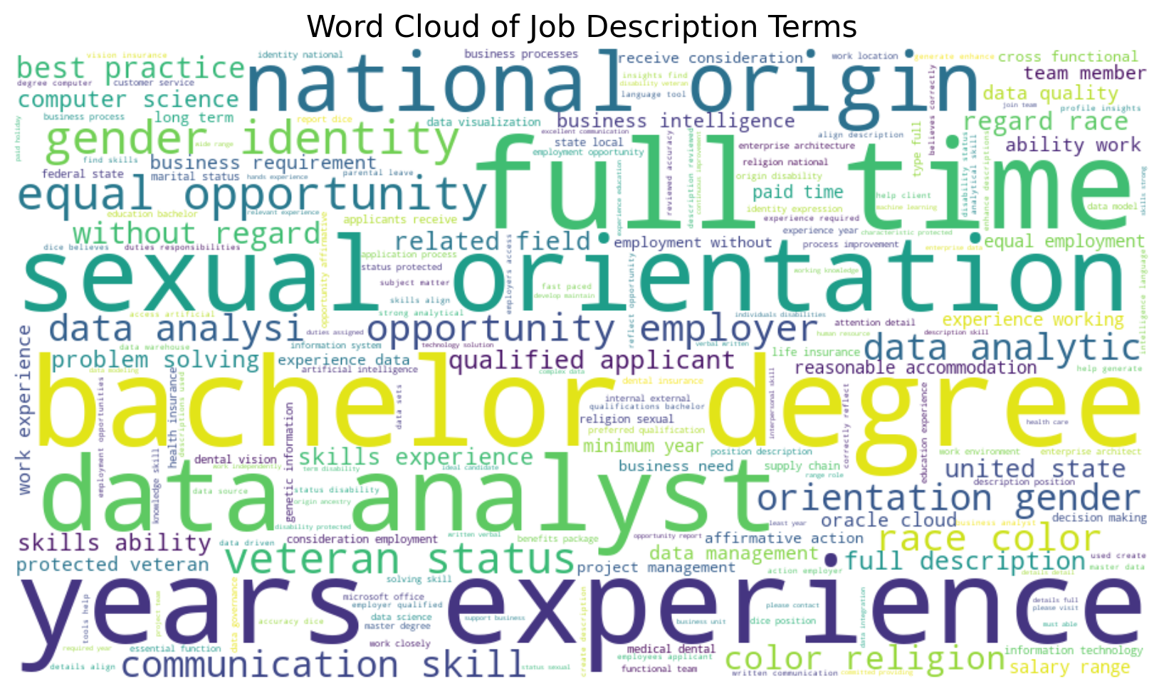
We aggregate a global vocabulary across all postings and compute the most frequently occurring terms.
A word cloud provides a quick, intuitive view of recurring terms. Large words appear more frequently in text, giving a qualitative impression of employer emphasis.
TF–IDF: High-Information Terms Across Job Descriptions
Raw word counts can be dominated by generic terms (for example, “team,” “support,” “experience”). To focus on high-information terms that distinguish postings, we apply TF–IDF (Term Frequency–Inverse Document Frequency).
This gives higher scores to words that
appear frequently within a posting, but
do not appear in every other posting.
Code
# For performance, optionally sample a subset if the dataset is hugeMAX_DOCS =15000iflen(df_text) > MAX_DOCS: df_tfidf = df_text.sample(n=MAX_DOCS, random_state=42).copy()else: df_tfidf = df_text.copy()tfidf_vectorizer = TfidfVectorizer( max_features=3000, min_df=5, max_df=0.6, stop_words=None# custom stopwords already applied at the text level)tfidf_matrix = tfidf_vectorizer.fit_transform(df_tfidf["clean_body"])feature_names = np.array(tfidf_vectorizer.get_feature_names_out())# tfidf_matrix.shape
Code
# Compute average TF–IDF score per term across all sampled documentsavg_tfidf = tfidf_matrix.mean(axis=0).A1tfidf_df = ( pd.DataFrame({"term": feature_names, "score": avg_tfidf}) .sort_values("score", ascending=False))# tfidf_top = tfidf_df.head(25)tfidf_df.head(3)
# Build separate corpora per sectorsector_texts = ( df_sector .groupby("sector")["clean_body"] .apply(lambda s: " ".join(s.tolist())))sector_texts
sector
Finance & Insurance                     taking care of people is at the heart of every...
Information                             about lumen lumen connects the world we are ig...
Professional, Scientific & Technical    sr marketing analyst united states ny new york...
Name: clean_body, dtype: object
Code
# Separate vectorizer for sector-level TF–IDFsector_vectorizer = TfidfVectorizer( max_features=2000, min_df=1, # allow terms that appear in at least one sector corpus max_df=1.0, # do not drop terms that appear across multiple sectors stop_words=None)sector_tfidf = sector_vectorizer.fit_transform(sector_texts.values)sector_terms = np.array(sector_vectorizer.get_feature_names_out())sector_tfidf.shape
(3, 2000)
Code
# For each sector, extract its top 15 TF–IDF termsrows = []for i, sector_name inenumerate(sector_texts.index): row_vec = sector_tfidf[i].toarray().ravel() top_idx = row_vec.argsort()[-15:][::-1]for idx in top_idx: rows.append({"sector": sector_name,"term": sector_terms[idx],"score": row_vec[idx] })sector_tfidf_df = pd.DataFrame(rows)sector_tfidf_df.head()
Although Lightcast provides structured software skill fields, job descriptions often repeat these terms inside free text. To quantify this, we scan cleaned descriptions for common technical keywords.
Global frequency and word clouds show recurring emphasis on experience, support, team, management, and responsibilities.
This indicates that employers value not only technical competence but also the ability to operate in collaborative, process-oriented environments.
High-Information Terms (TF–IDF)
TF–IDF surfaces more specialized vocabulary (e.g., “pipeline,” “analytics,” “visualization,” “governance”) that differentiates advanced analytics roles from generic postings.
These terms often correspond to specific project responsibilities or technical domains within data teams.
Sector-Specific Vocabulary
In Finance & Insurance, TF–IDF highlights concepts related to risk, portfolios, credit, and regulatory reporting.
In Professional, Scientific & Technical Services, terms linked to modeling, experimentation, and client delivery become more prominent.
In Information, we see emphasis on platforms, content, and digital products.
This demonstrates how sector context shapes the language of “data work.”
Technical Signal in Text
The repeated presence of terms such as SQL, Python, Excel, Tableau, Power BI, AWS, and Azure inside descriptions reinforces the structured skill patterns observed in the EDA section.
These technologies function as “linguistic anchors” that clearly distinguish analytics roles from general business positions.
Implications for Job Seekers
Candidates aligning with these text-level signals (SQL + Python + BI + cloud) are better positioned for data-intensive roles.
Beyond tools, employers repeatedly emphasize concepts related to analysis, insights, decision-making, and stakeholder communication — confirming that soft skills and interpretation capabilities matter as much as raw coding ability.
Understanding how employers write about roles helps job seekers tailor resumes, cover letters, and LinkedIn profiles using the same vocabulary that appears in successful job descriptions.
Taken together, the NLP results provide a qualitative, language-based complement to our structured EDA and Skill Gap Analysis, strengthening the case for a hybrid skill profile: technical depth, sector awareness, and communication skills that translate data into decisions.